Week 6: Conjugate Heat Transfer Simulation
AIM
To conduct conjugate heat transfer simulation in converge
OBJECTIVES
Grid dependence test
- Start with an initial base grid
- Run grid dependence test on 3 grids and show that the outlet temperature converges to a particular value
Effect of supercycle stage interval
- Set supercyle stage interval to 0.01,0.02 and 0.03
- For these three values, how does the total simulation time compare against the baseline configuration
THEORY
Conjugate Heat Transfer (CHT)
The term Conjugate Heat Transfer (CHT) is used to describe processes that involve simultaneous energy exchange between the solid and fluid domains due to interaction between them and is frequently encountered in a variety of engineering applications such as internal combustion engines, turbo-machinery, heat exchangers, etc.
The Conjugate Heat Transfer (CHT) analysis type allows for the simulation of heat transfer between solid and fluid domains by exchanging thermal energy at the interfaces between them. Typical applications of this analysis type exist as, but are not limited to, the simulation of heat exchangers, cooling of electronic equipment, and general-purpose cooling and heating systems. Computational Fluid Dynamics (CFD) and more specifically conjugate heat transfer (CHT) analysis can accurately predict heat transfer by simultaneous solving all the relevant solid and flow field heat transfer processes.
It represents a class of multi-physics problems where fluid flow affects the thermal behaviour of structure, which in turn affects the fluid flow. For conjugate heat transfer analyses, the solid material conduction and the fluid convection are analysed simultaneously. The conductive heat transfer in a solid region is coupled to the convective heat transfer in a neighbouring fluid flow.
Supercycling
Supercycling is a strategy in converge for accelerating CHT calculations. CONVERGE offers an approach called super-cycling for overcoming the time-scale disparity. In super-cycling, the fluid solver is frozen periodically while the heat transfer in the solid is allowed to progress to steady-state. CONVERGE solves the fluid and solid phases in the same simulation without requiring you to stop and restart the simulation. Super-cycling significantly reduces the computational cost of the CHT simulation.
SIMULATION PROCEDURE
- Setting up the case in converge
- Running the simulation in cygwin
- Post convert using cygwin/converge
- Post processing in paraview
The first step is case setup in converge. Open converge and then create the geometry.
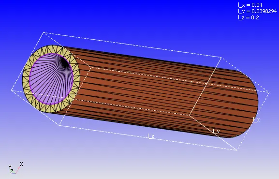
Geometry dimensions
Inner diameter = 0.03m
Thickness diameter = 0.01m
Length of pipe = 0.2m
Flag the boundaries
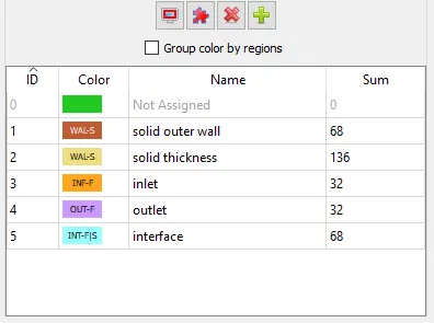
After that check the orientation of normal and run a diagnosis check.
The next step is case setup.
Inorder to run a transient state simulation firstly under application type in the setup tree, a time based simulation must be selected. Then click on materials and select air to predefined mixtures.
Enable solid simulation and species. In gas simulation retain the default settings.
In solid simulation add aluminium.
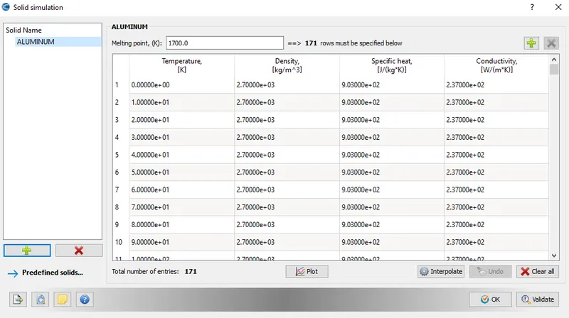
Open the species tab, add aluminium as solid species and add O2 and N2 as gas species.
Run parameters
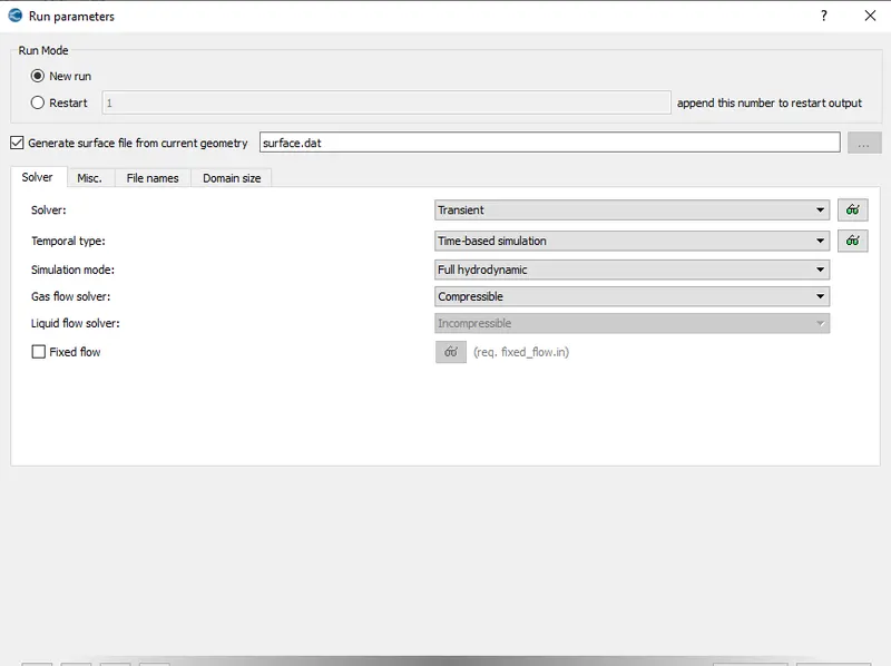
Simulation time parameters
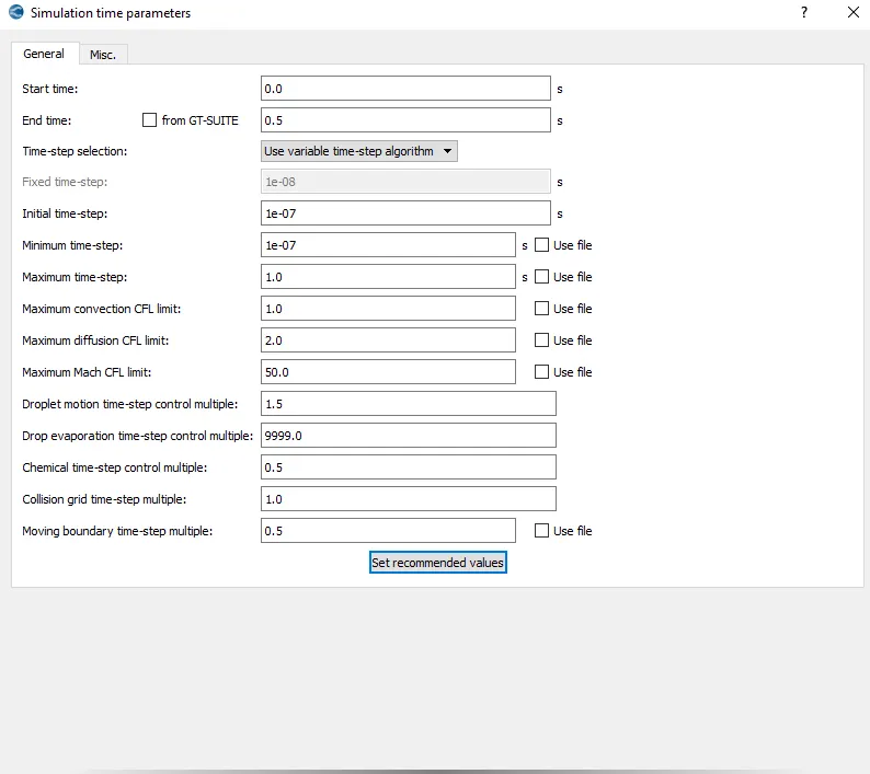
In solver parameters retain the default setting.
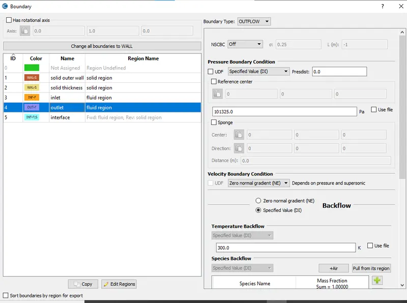
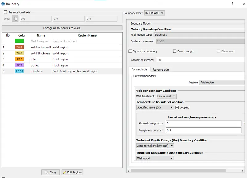
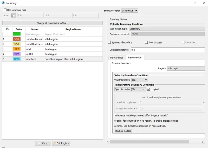
Give the boundary conditions as given below
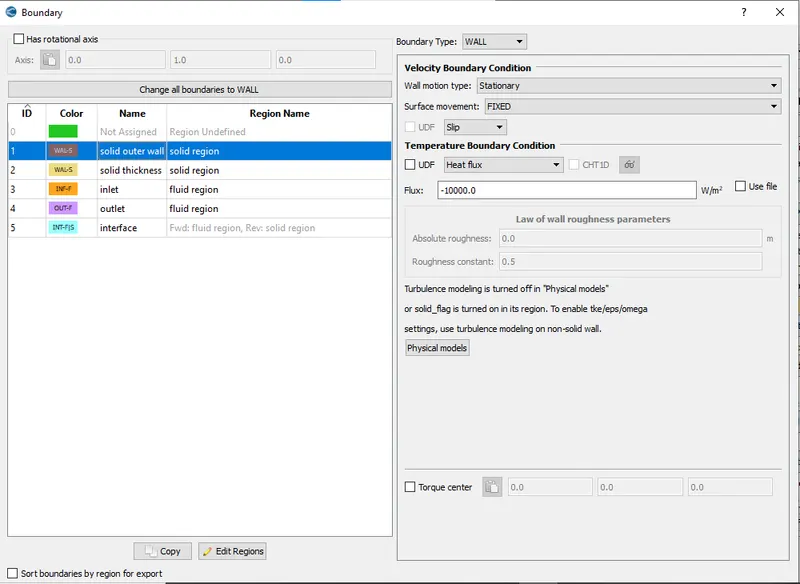
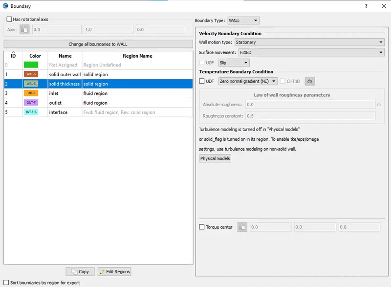
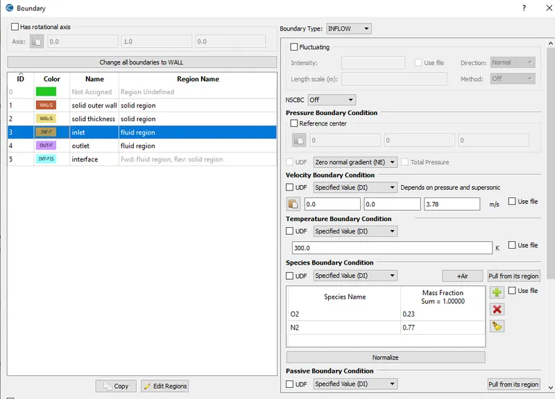
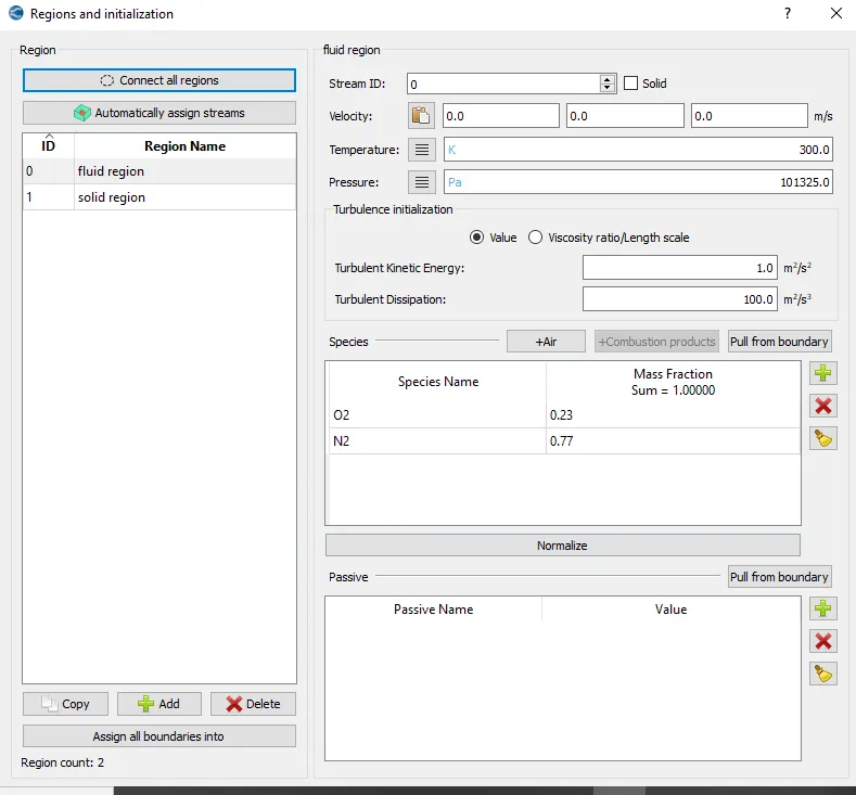
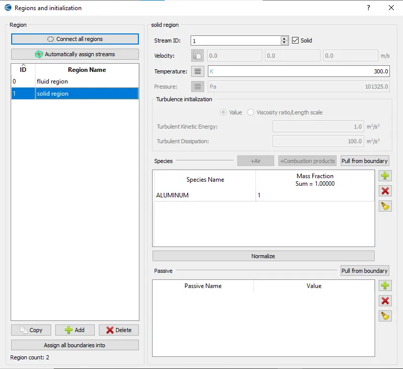
Regions and Initialisation
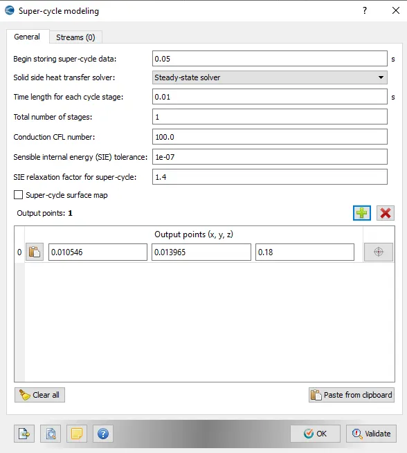
In physical models, enable Turbulence modelling and super cycle modelling.
Retain the default setting for turbulence modelling.
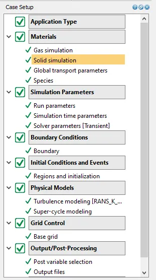
Once the case setup is completed, export the input files into a required directory. Then launch cygwin and navigate to the directory through CYGWIN in which all input files has been exported and then enter the command to run the simulation ' mpiexec.exe -n 1 converge.exe restricted'. After that post convert using converge and post process the results in paraview.
RESULTS
Re = (rho*V*D)/(Dynamic viscosity)
Velocity, `V = (Re*mu)/(rho*D`
`V = (7000*0.00001846)/(1.171*0.0299)`
`V = 3.78 m/s`
Grid dependence test
Case 1
mesh size = 1mm
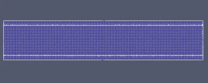
Mesh
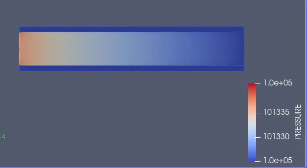
Pressure contour
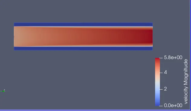
Velocity contour
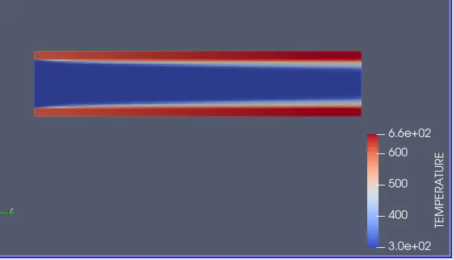
Temperature contour
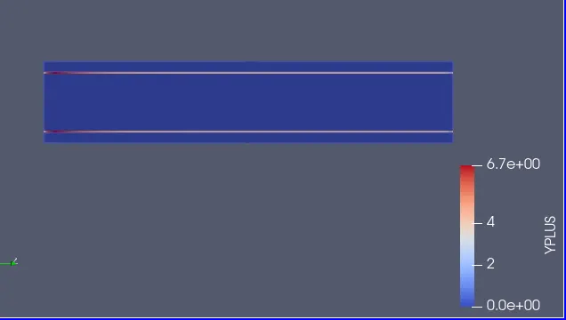
Yplus
Temperature animation
Case 2
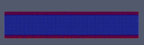
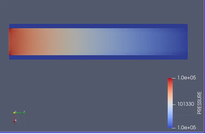
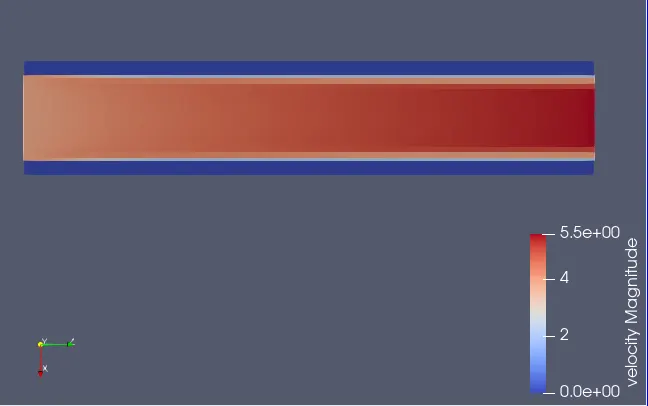
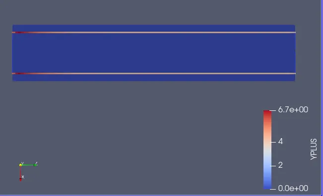
mesh size = 2mm
Mesh
Pressure
Velocity
Yplus
Temperature animation
Case 3
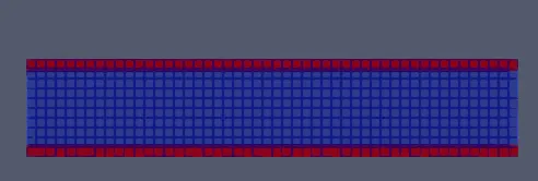
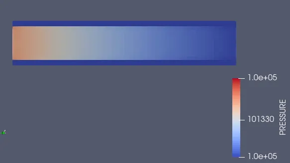
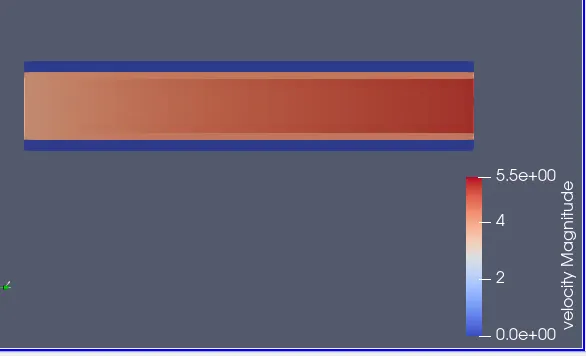
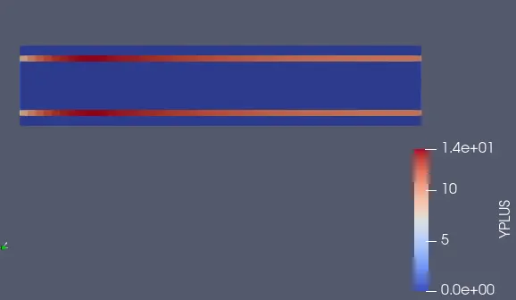
mesh size = 4mm
Mesh
Pressure
Velocity
Yplus
Temperature animation
From the results, we can see that there is only a small variation in the values as the mesh size increases.With mesh refinement the results are much smoother.
Effect of supercycle stage interval
Fluid region
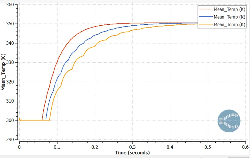
The red line indicates the fluid region region mean temperature for supercycle stage interval 0.01s. We can see that this curve converges faster compared to the others and the curve is smoother. That is for fluid region the curve attains convergence faster for lower value of supercycle stage interval.
Solid region
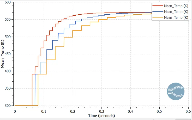
For solid region, the curve which represents the supercycle stage interval value of 0.01s (red line), converges faster compared to others. Since the time length for each cycle stage is smaller (0.01s) the solid domain is solved more number of times and convergence is attained faster compared to other supercycle stage intervals. So supercycling helps to speed up the simulation. In this plot for solid region we can see the temperature is jumping suddenly which results in step-like graph. This is because of supercycling, the solver for the fluid domain is paused until the solid domain converges. This pausing is done in intervals. The jumps in the plot represent the updation of the solid temperature.
| Super cycling stage interval(s) | Grid size(mm) | Time (s) |
| 0.01 | 4mm | 263s |
| 0.02 | 4mm | 287s |
| 0.03 | 4mm | 302s |
As the supercycling stage interval decreases from 0.03 to 0.01, the computational time decreases.
CONCLUSION
- The conjugate heat transfer simulation of flow through a pipe was conducted using converge CFD. A grid independency test was conducted and effect of supercycle stage interval was studied.
- The refinement of mesh results in more accurate results but with the expense of computational time.
- Decreasing the supercycle stage interval helps to reduce the computational time and produces more smoother results.