Week 7: Shock tube simulation project

AIM

To simulate shock tube using converge

OBJECTIVES

• Setup a transient shock tube simulation
• Plot the pressure and temperature history in the entire domain
• Plot the cell count as a function of time

THEORY

Shock tube

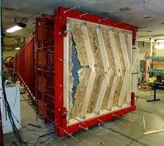
The shock tube is an instrument used to replicate and direct blast waves at a sensor or a model in order to simulate actual explosions and their effects, usually on a smaller scale. Shock tubes (and related impulse facilities such as shock tunnels, expansion tubes, and expansion tunnels) can also be used to study aerodynamic flow under a wide range of temperatures and pressures that are difficult to obtain in other types of testing facilities. Shock tubes are also used to investigate compressible flow phenomena and gas phase combustion reactions. More recently, shock tubes have been used in biomedical research to study how biological specimens are affected by blast waves. A shock wave inside a shock tube may be generated by a small explosion (blast-driven) or by the buildup of high pressures which cause diaphragm to burst and a shock wave to propagate down the shock tube (compressed-gas driven).

SIMULATION PROCEDURE

1. Setting up the case in converge
2. Running the simulation in cygwin
3. Post convert using cygwin/converge
4. Post processing in paraview

The first step is case setup in converge. Open converge and then import the geometry.

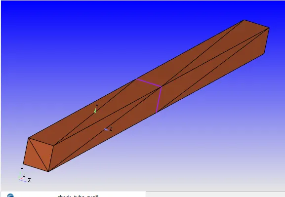
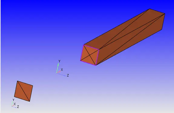
There is a diaphragm present inside the geometry. To avoid the non-manifold edges the diaphragm must be deleted.

Name the boundaries

The orientation of normals should be checked such that it should be pointing towards the flow.

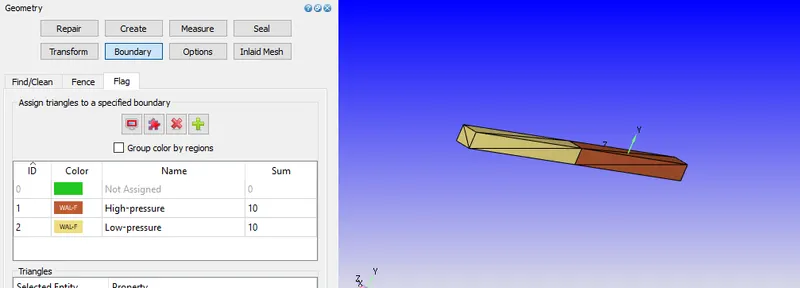
Then run a diagnosis check to find if there are any errors.

Geometry preparation is completed. The next step is case setup.

Inorder to run a transient state simulation firstly under application type in the setup tree, a time based simulation must be selected.

In materials turn on species and in predefined mixtures select air.

In gas simulation and global transport properties, default properties are maintained.

In species tab, add O2 and N2.

The next one in the case setup tree is the simulation parameters.

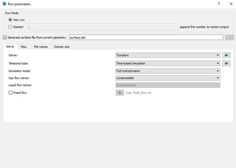
In run parameters, transient solver is selected.

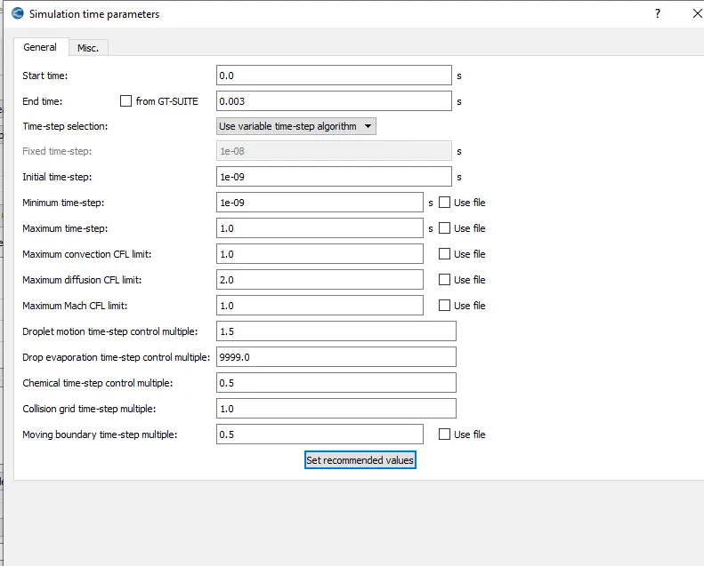
Set the simulation time parameters

In solver parameters, keep all settings as default.

Give the boundary conditions as given below.

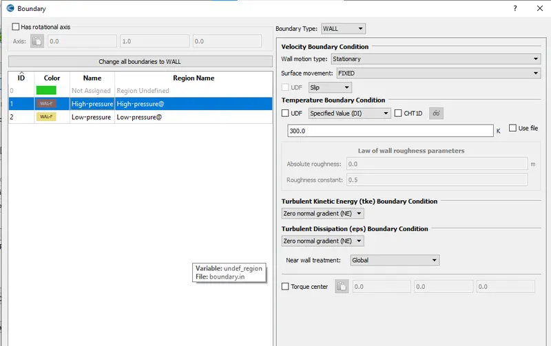
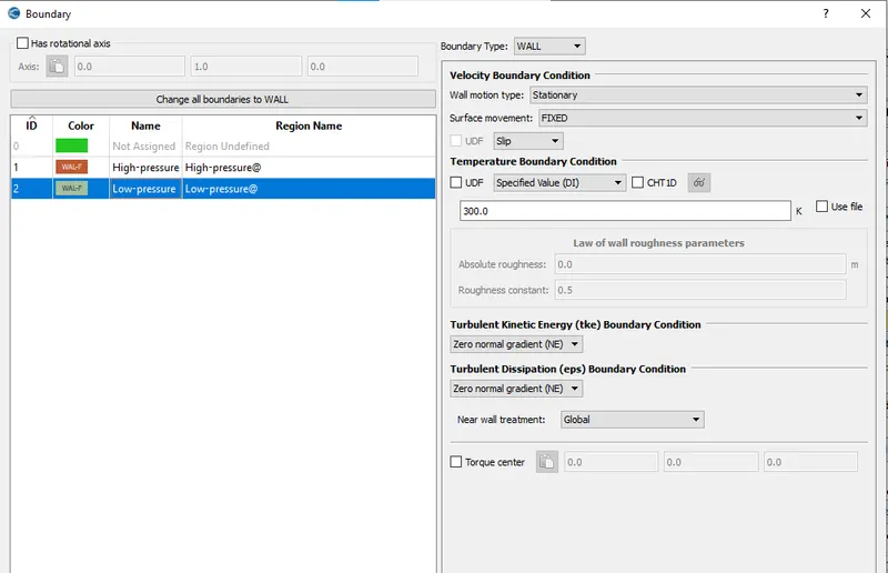
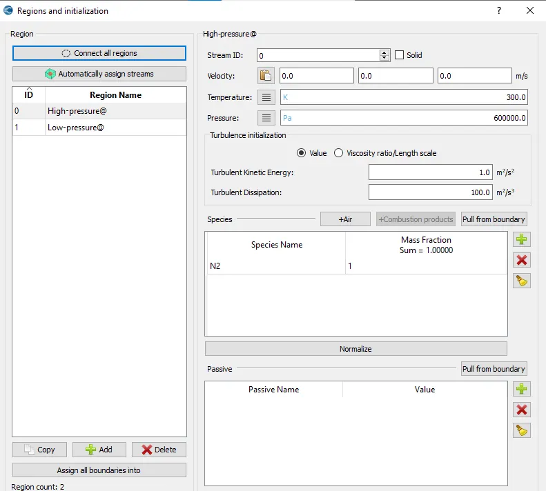
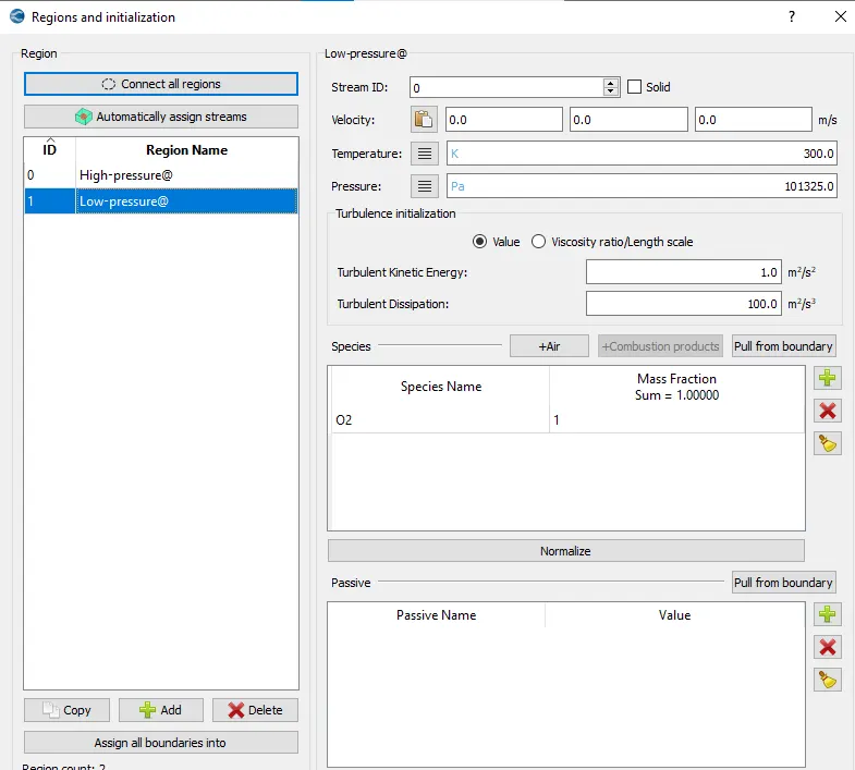
In Regions and Initialisation, two regions are created.

High pressure region with temperature 300k

Pressure 600000 Pa

Species N2 with mass fraction 1

Low pressure region with temperature 300k

Pressure 101325 Pa

Species O2 with mass fraction 1

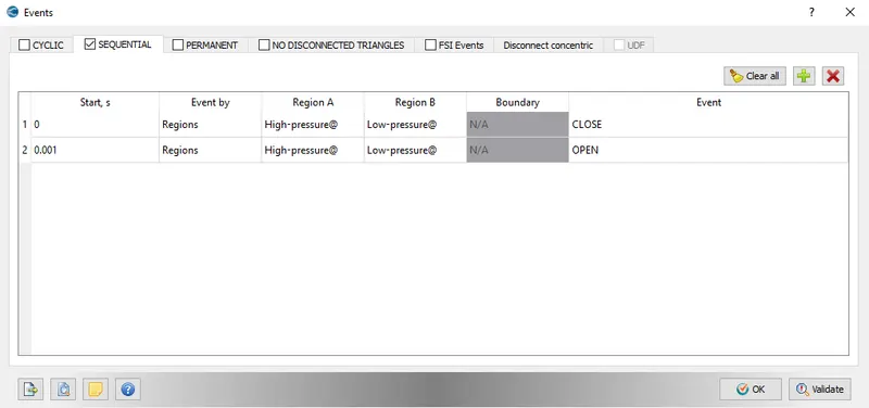
When two regions are in contact with each other with no boundary in between them, it is necessary to use events. The event flag creates triangles in between the two regions called as disconnect triangles. With the help of events we can connect or disconnect the two regions.

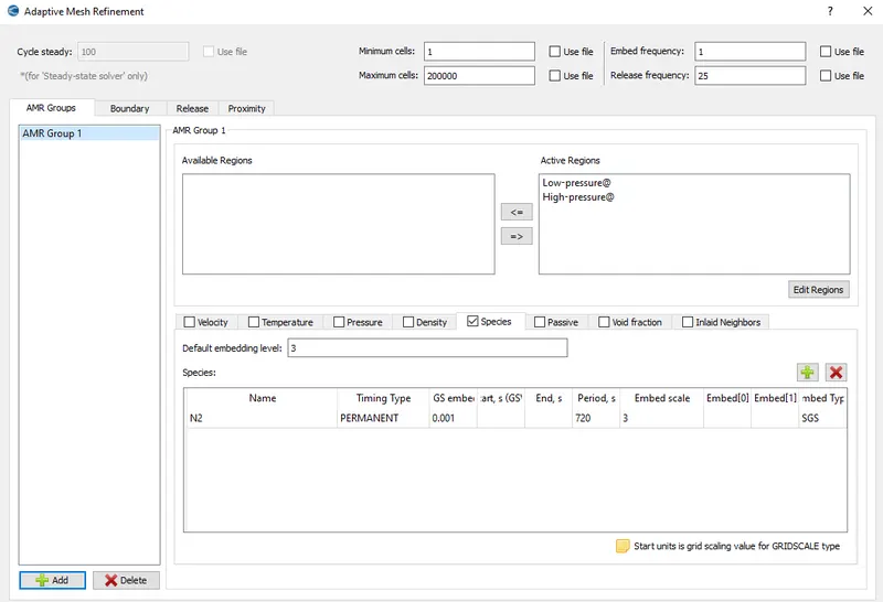
In turbulence modeling keep all the default settings. In grid control enable adaptive mesh refinement.

The base grid size is 0.002m.

In AMR give the settings as given below. Species scheme is used for AMR.

Set the frquency of generation of output files.

Once the case setup is completed, export the input files into a required directory. Then launch cygwin and navigate to the directory through CYGWIN in which all input files has been exported and then enter the command to run the simulation ' mpiexec.exe -n 1 converge.exe restricted'. After that post convert using converge and post process the results in paraview.

RESULTS

Mesh

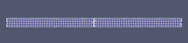
Adaptive mesh refinement

https://drive.google.com/file/d/1Z1vqpR8Tcen841RGbJgdsYEmKB13fm9F/view?usp=sharing

Total cell count plot

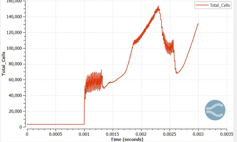
In the events option the bursting of diaphragm was set at 0.001seconds. After that we can see the variation in the number of cells. This is because as the diaphragm bursts the high pressure region pushes the low pressure region and the AMR gets activated.

Tempreature contour

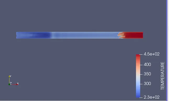
The temperature throughout the shock tube initially is 300k. After the shock waves start propogating the temperature starts varying. This can be seen from the animation video provided below.

Temperature animation

https://drive.google.com/file/d/1Jc_5_H47DPHshOt99l-OXahaMX6yE0Xi/view?usp=sharing

Pressure contour

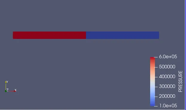
The flow is static before the event occurs, because the two regions are closed. After 0.001s two regions get opened and the flow takes place high pressure region to low pressure region. Due to the instantaneous compression of the gas, shock develops. Then shock waves get reflect from the walls resulting in refraction waves.

Pressure animation

https://drive.google.com/file/d/1UpGicGqfsd_gHelaxHKy0kUi9S3r0J1y/view?usp=sharing

Velocity animation

https://drive.google.com/file/d/1KNjffX4Vc4jw7qwo0JJmD0WnbINRB0eG/view?usp=sharing

CONCLUSION

• Shock tube simulation was conducted in ansys fluent.
• Using events option the flow was set to propogate after 0.001s. In this way diaphragm bursting was mimicked.
• With adaptive mesh refinement shock propogation was captured.