Week 9 - FVM Literature Review

AIM

What is Finite Volume Method(FVM), write down the major differences between FDM & FVM. Also, describe the need for interpolation schemes and flux limiters in FVM.

Finite Volume Method

The Finite Volume Method (FVM) is a discretization method for the approximation of a single or a system of partial differential equations expressing the conservation, or balance, of one or more quantities. These partial differential equations (PDEs) are often called conservation laws; they may be of different nature, e.g. elliptic, parabolic or hyperbolic, and they are used as models in a wide number of fields, including physics, biophysics, chemistry, image processing, finance, dynamic reliability. They describe the relations between partial derivatives of unknown fields such as temperature, concentration, pressure, molar fraction, density of electrons or probability density function, with respect to variables within the domain (space, time,...) under consideration. The FVM is based on the fact that many physical laws are conservation laws—what goes into one cell on one side needs to leave the same cell on another side. Following this idea, you end up with a formulation that consists of flux conservation equations defined in an averaged sense over the cells. Historically, this method has been very successful in solving fluid flow problems

The FVM is a method for representing and evaluating partial differential equations in the form of algebraic equations. In the finite volume method, volume integrals in a partial differential equation that contain a divergence term are converted to surface integrals, using the divergence theorem. These terms are then evaluated as fluxes at the surfaces of each finite volume. Because the flux entering a given volume is identical to that leaving the adjacent volume, these methods are conservative. Another advantage of the finite volume method is that it is easily formulated to allow for unstructured meshes. The method is used in many computational fluid dynamics packages. "Finite volume" refers to the small volume surrounding each node point on a mesh.

Finite volume methods can be compared and contrasted with the finite difference methods, which approximate derivatives using nodal values, or finite element methods, which create local approximations of a solution using local data, and construct a global approximation by stitching them together. In contrast a finite volume method evaluates exact expressions for the average value of the solution over some volume, and uses this data to construct approximations of the solution within cells.

Major differences between FDM & FVM

• The finite-difference method is defined dimension per dimension; this makes it easy to increase the “element order” to get higher-order accuracy. If you can fit the simulation in a rectangular or box-shaped geometry using a regular grid, efficient implementations are much easier than for finite-element and finite-volume methods.
• The finite-difference method is more difficult to use for handling material discontinuities. In addition, it does not lend itself for local grid refinement or anything similar to “adaptive mesh refinement.” This may be needed to resolve local rapid variations in solutions such as around a corner of a complex shape.
• The finite-volume method is a natural choice for CFD problems, since the partial differential equations you have to solve for CFD are conservation laws. However, both finite differences and finite elements can also be used for CFD. Techniques for CFD with the finite-difference and finite-volume method have been known and used much longer.
• 
  The finite-volume method’s strength is that it only needs to do flux evaluation for the cell boundaries. This also holds for nonlinear problems, which makes it extra powerful for robust handling of (nonlinear) conservation laws appearing in transport problems.
• The local accuracy of the finite-volume method, such as close to a corner of interest, can be increased by refining the mesh around that corner, similar to the finite-element method. However, the functions that approximate the solution when using the finite-volume method cannot be easily made of higher order. This is a disadvantage of the finite-volume method compared to the finite-difference method.

Need for interpolation schemes and flux limiters in FVM

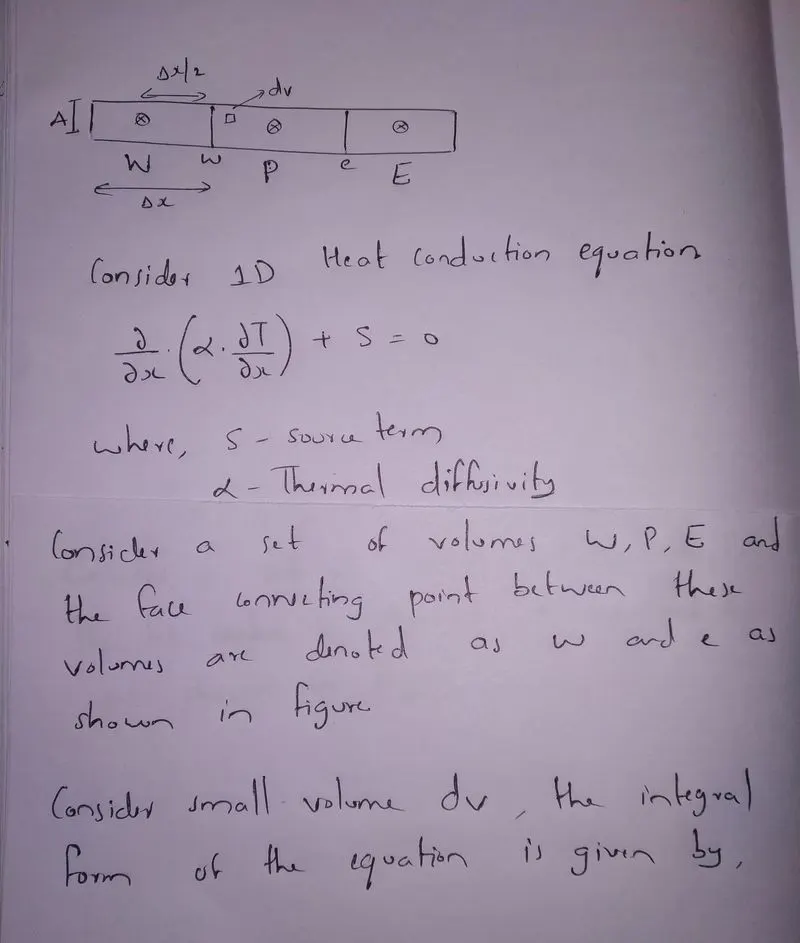
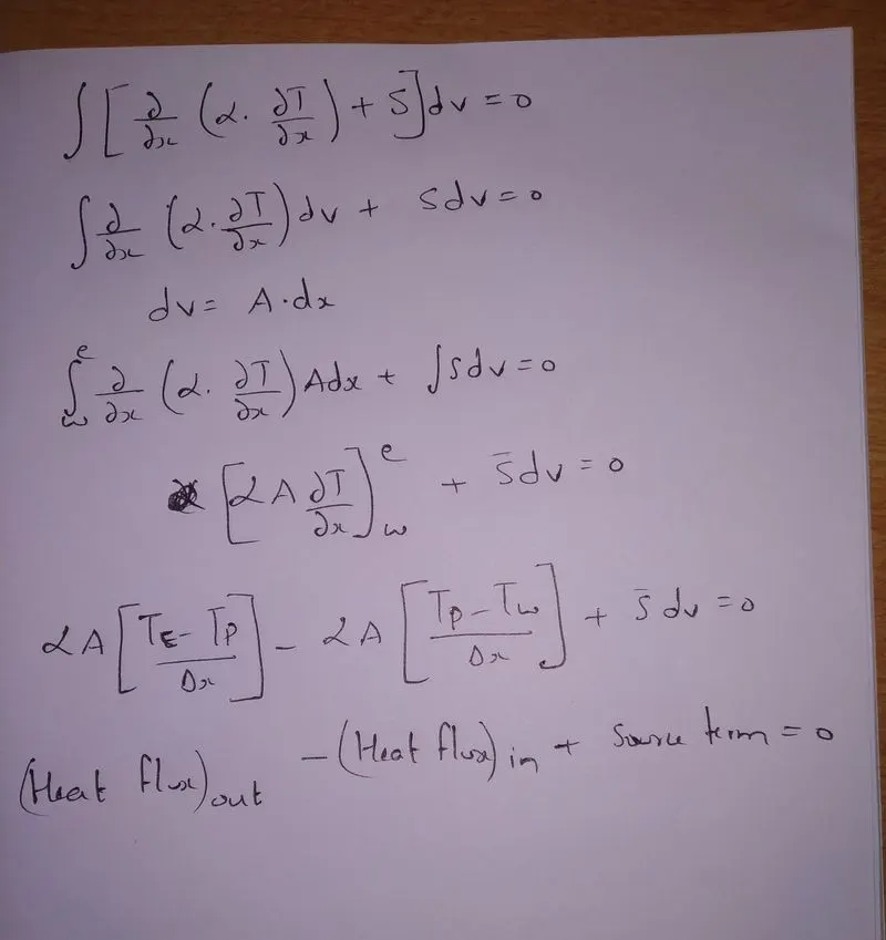
The interpolation schemes are used to find the temperature values at `T_e` and `T_w`, since we know the values at `T_P, T_W, T_E`.

Interpolation schemes are used to transform cell-centre quantities to face centres. The operation is used in many of the finite volume calculations, e.g. for the calculation of gradient, divergence, and Laplacian terms. A wide variety of interpolation schemes are available, ranging from those that are based solely on geometry, and others, e.g. convection schemes that are functions of the local flow.

Flux limiters are used in high resolution schemes – numerical schemes used to solve problems in science and engineering, particularly fluid dynamics, described by partial differential equations (PDE's). They are used in high resolution schemes, to avoid the spurious oscillations (wiggles) that would otherwise occur with high order spatial discretization schemes due to shocks, discontinuities or sharp changes in the solution domain. Use of flux limiters, together with an appropriate high resolution scheme, make the solutions total variation diminishing (TVD).

Most of us might have seen the behaviour of numerical schemes in order to capture shocks and discontinuity that arises in hyperbolic equations. Physically, these equations model the convective fluid flow. It has been observed that low-order schemes are usually stable but quite dissipative in nature around the points of discontinuity/shocks. One can not have high order accuracy without oscillations. The objective is to have highly accurate and stable oscillation free schemes. This kind of schemes are known as high resolution schemes.
Here we talk only about using flux limiters function to construct high resolution schemes. The idea is to tune the numerical flux of high order and low order scheme using the flux limiter function in such a way that the resulting scheme gives a high order accuracy in the smooth region of flow and sticks with first order of accuracy in the vicinity of shocks/discontinuities.

The flux limiters are also referred to as slope limiters because they both have the same mathematical form, and both have the effect of limiting the solution gradient near shocks or discontinuities. In general, the term flux limiter is used when the limiter acts on system fluxes, and slope limiter is used when the limiter acts on system states (like pressure, velocity etc.).