Week 1- Mixing Tee

AIM

Setup steady state fluent simulations in Ansys to compare the mixing effectiveness for short and long pipes.

OBJECTIVES

• Set up steady-state simulations to compare the mixing effectiveness when hot inlet temperature is 36⁰C & the Cold inlet is at 19⁰C
• Compare K epsilon and K omega SST model and based on the results choose which is suitable for this project
• Show the convergence plot for each case
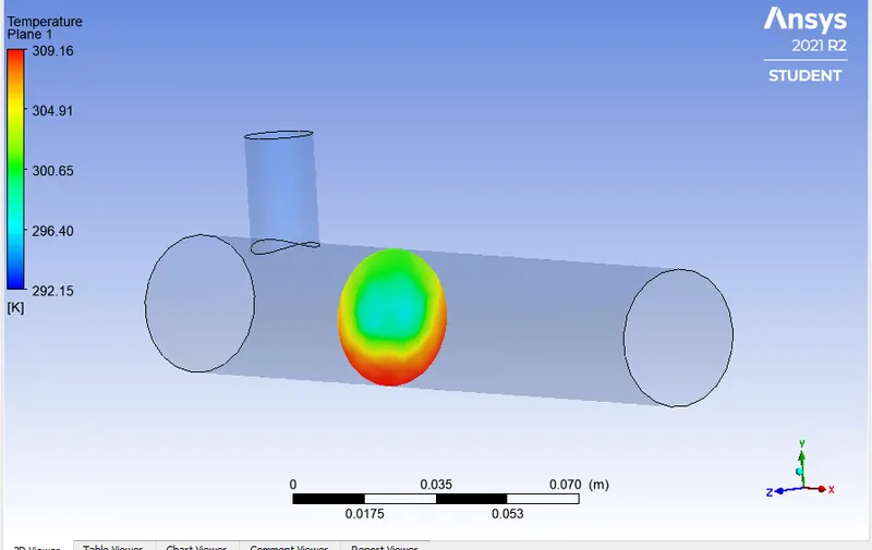
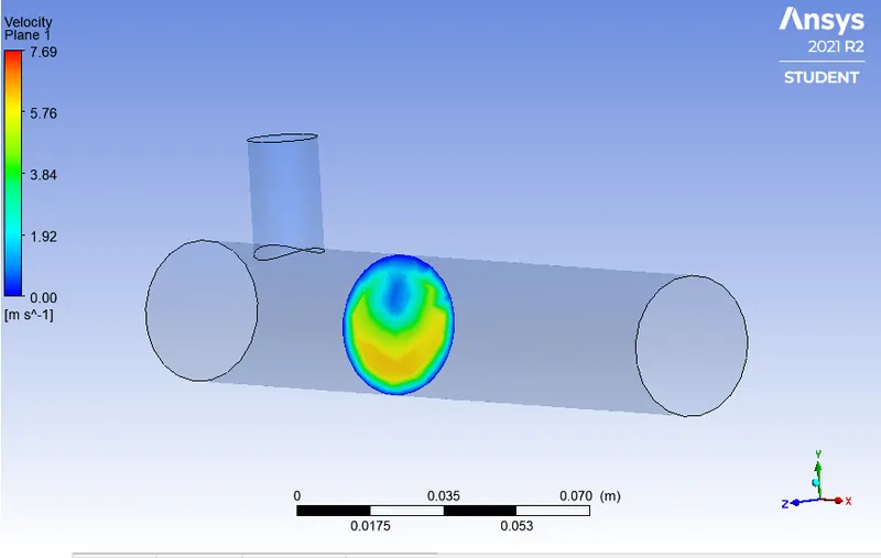
• Plot the velocity and temperature contour plots on the cut planes along and across the pipe.
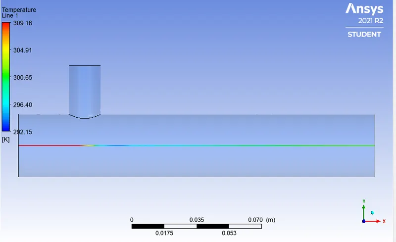
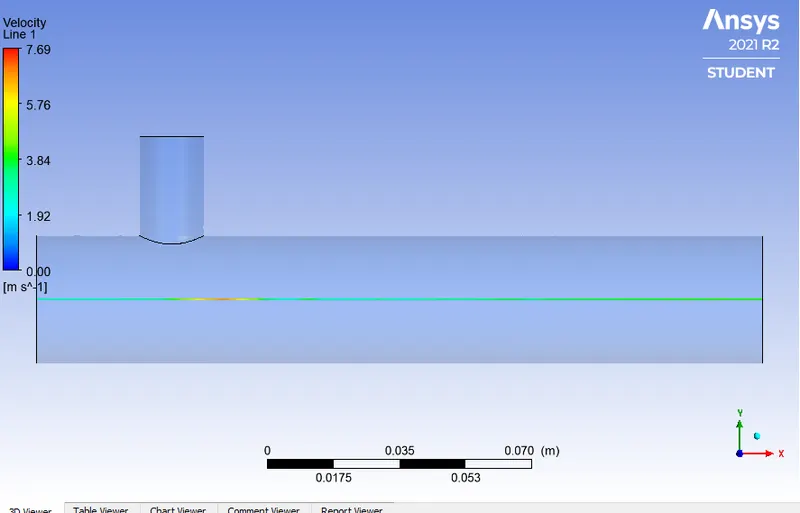
• Plot the velocity and temperature line plots along and across the length of the pipe.
• Perform mesh independence study for any one case
• Discuss the effect of length and momentum ratio on results

The objective is to create fluent simulations for two versions of the mixing tee, one of them is longer than the other.

1. Case 1
   • Short mixing tee with a hot inlet velocity of 3m/s.
   • Momentum ratio of 2, 4.
2. Case 2
   • Long mixing tee with a hot inlet velocity of 3m/s.
   • Momentum ratio of 2, 4.

Momentum ratio = velocity at cold inlet / velocity at hot inlet

Mixing tees

Mixing Tees utilizes a specifically engineered internal geometry to efficiently mix two fluid streams into one combined stream. These mixing tees are specifically designed for high pressure applications. Mixing tees in which two fluid streams with different physical and/or chemical properties mix are widely used in the petrochemical industry. When there is a large temperature difference between two streams, large metal temperature fluctuations can occur in the region where the two streams meet if proper design steps are not taken. The temperature fluctuations in the metal can lead to thermal fatigue of the pressure boundary piping. If through-wall cracking occurs, the fluid may leak, possibly causing a fire and damage. Therefore, it is imperative to ensure that the piping system can withstand the temperature fluctuations. Options can include improving the mixing of the two streams to reduce the temperature fluctuations through redesign of the piping system such that the momentum ratio of the two fluid streams is favorable to rapid mixing, or installing devices that protect the pressure boundary piping.

The first step is to find which method is better: K-epsilon or K-omega SST model

For both models the hot inlet velocity is set as 3m/s and cold inlet velocity as 6m/s

Hot inlet temperature is 36⁰C & the Cold inlet is at 19⁰C

Short mixing tee is selected

K epsilon

The k-epsilon model for turbulence is the most common to simulate the mean flow characteristics for turbulent flow conditions. It belongs to the Reynolds-averaged Navier Stokes (RANS) family of turbulence models where all the effects of turbulence are modeled. It is a two-equation model.

K omegs SST

The SST k-omega turbulence model is a two-equation eddy-viscosity model that is used for many aerodynamic applications. It is a hybrid model combining the Wilcox k-omega and the k-epsilon models. The k-omega model is well suited for simulating flow in the viscous sub-layer.

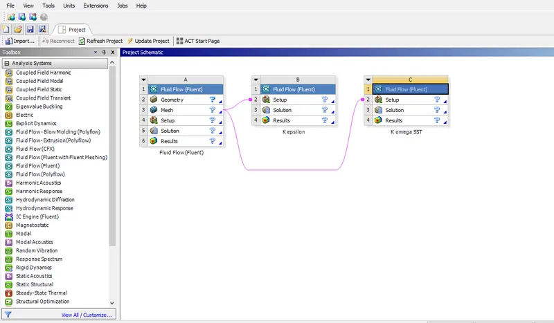
Open Ansys workbench and choose analysis system 'Fluid flow(fluent)'. Same geometry and mesh is used for both models.

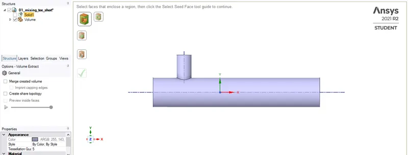
First the geometry is to be created in spaceclaim

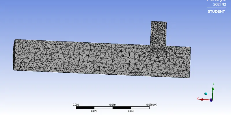
Then mesh is created

Double click on setup, then CFD solver will open.

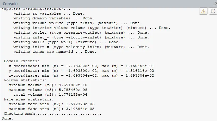
Check the mesh quality

Change the unit ot temperature to celsius. Then set up the physics of the domain as shown below;

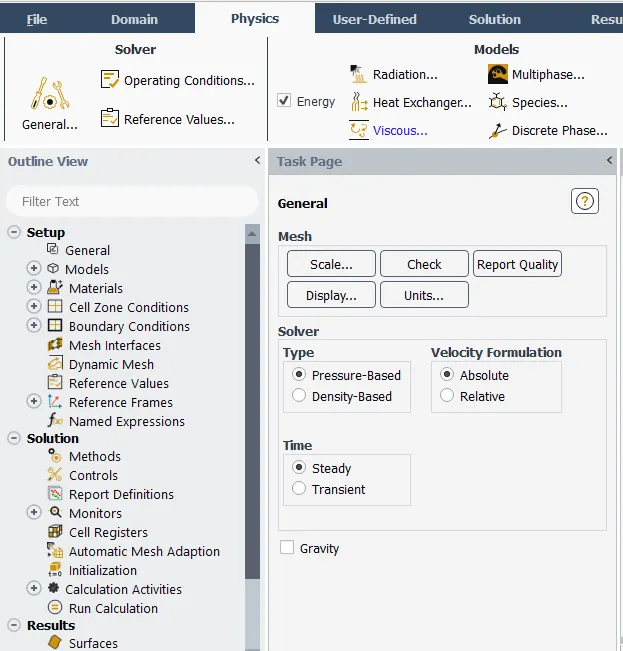
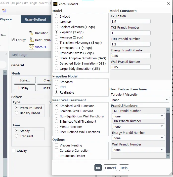
Turn on energy equation. In viscous model select K epsilon Realizable model.

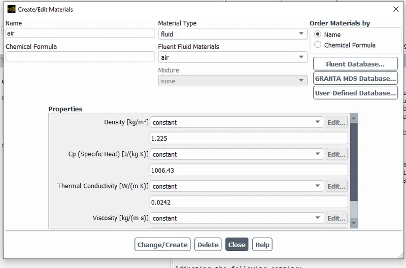
Click on materials and set the working fluid as air. (The working fluid is set as air by default)

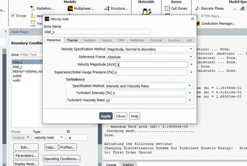
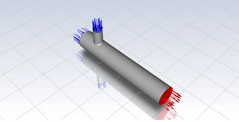
In zones set the cell zones and boundaries. Setup the boundary conditions for all boundaries. In boundary condition click on inlet x and set the velocity and temperature as required. Similary do this for inlet y and set outlet pressure condition as atmospheric pressure value.

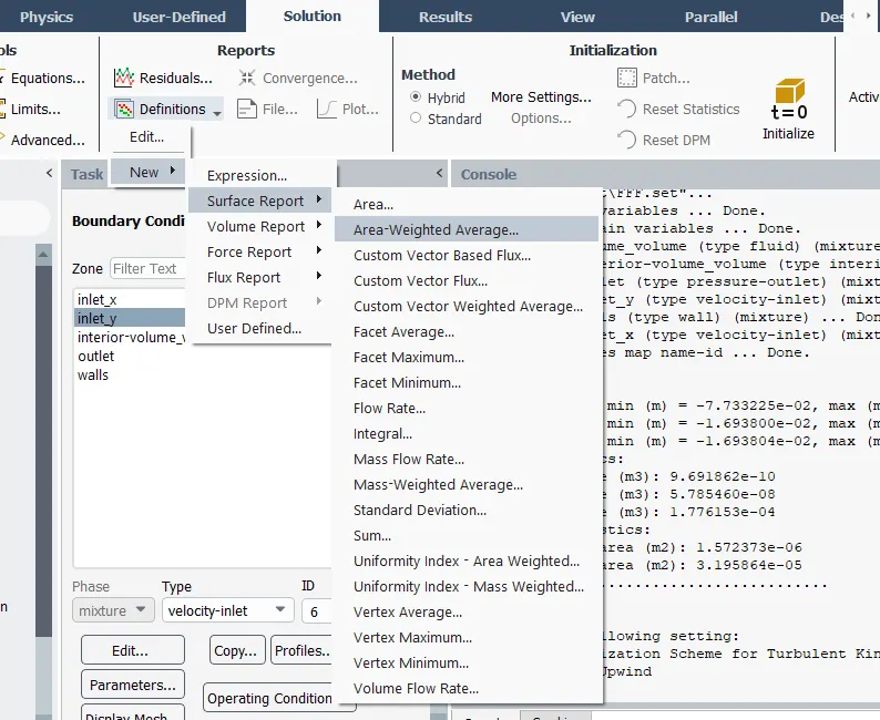
In reports click on definitions and add 2 reports - Area weighted average of temperature and Standard deviation of temperature for outlet

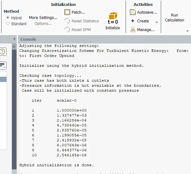
In initialization click on Hybrid initialization and then click on initialize

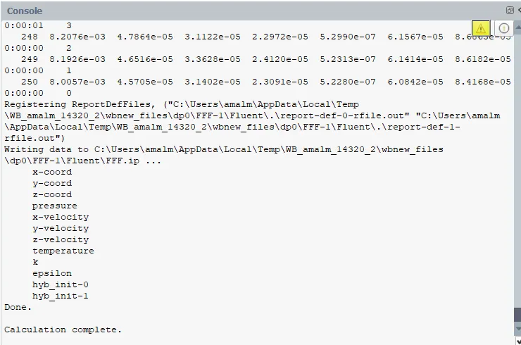
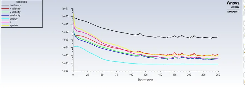
Then run the calculation for 250 iterations

Mesh

Convergence plot

Area weighted average of temperature at oulet for each iterations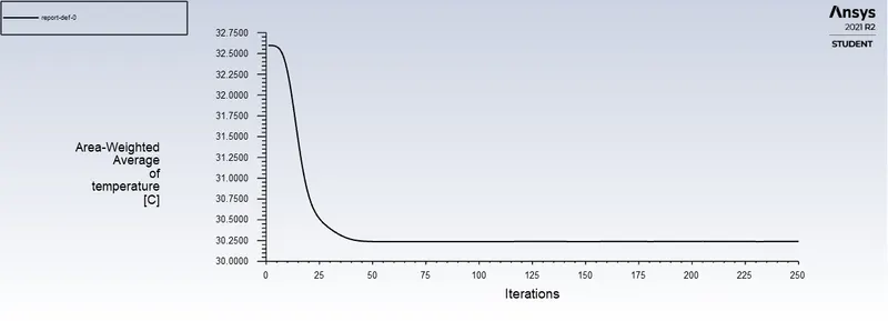

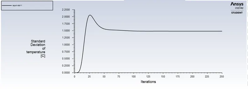
Standard deviation of temperature at oulet for each iteration

Close the fluent and click on results in workbench which will open CFD-post.

Click on the walls and decrease its transparency.

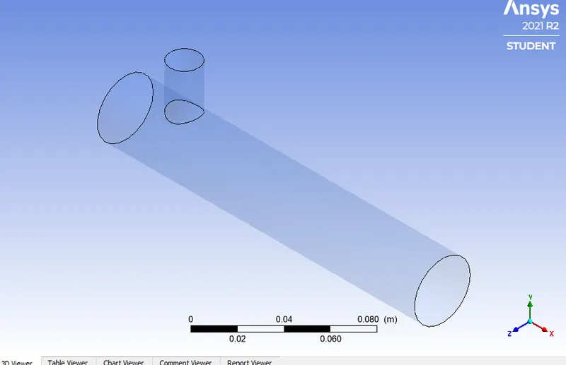
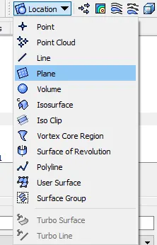
Create a plane by clicking on location and select plane, set method to be YZ plane.

Then create velocity and temperature contour plots

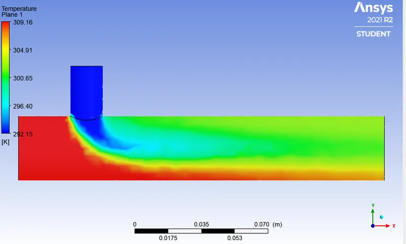
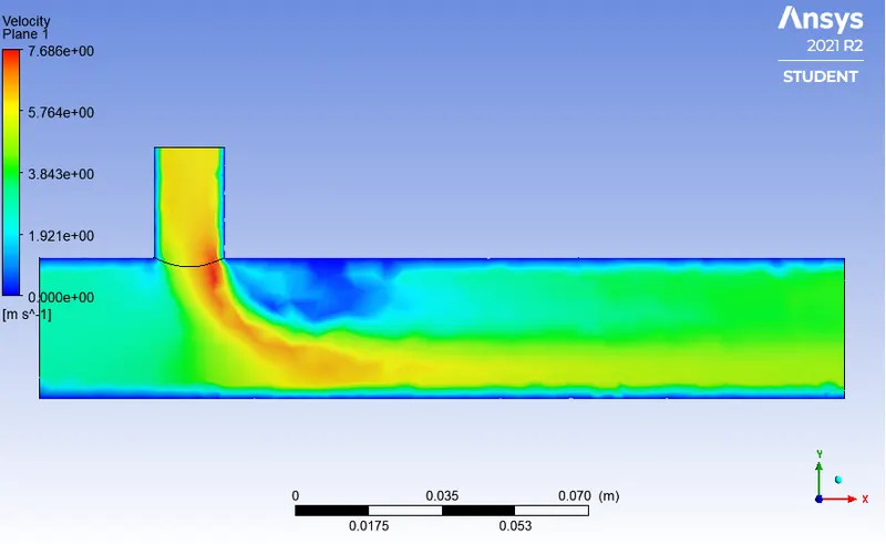
Computational time required for k epsilon model = 50 sec

Similarly create the results for K omega SST model.

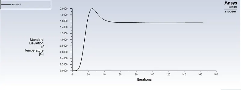
Convergence plot

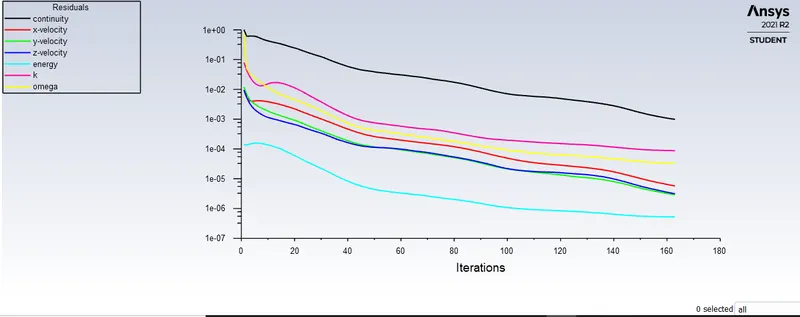
Area weighted average of temperature at oulet for each iterations

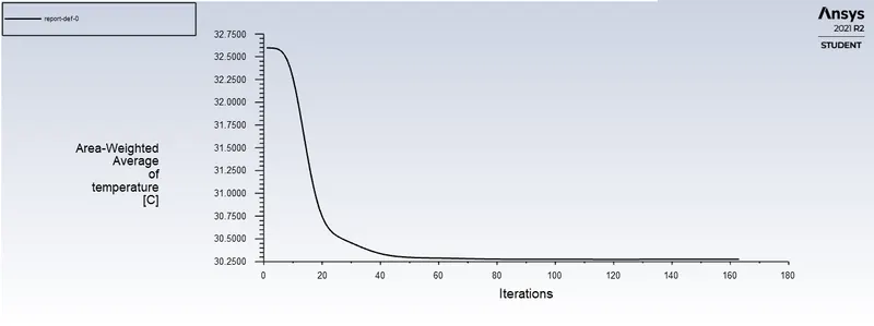
Standard deviation of temperature at oulet for each iteration

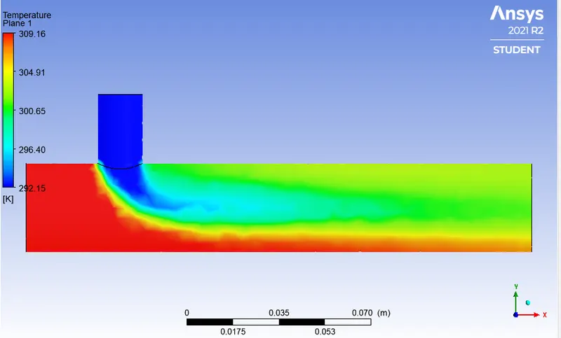
Temperature contour plot

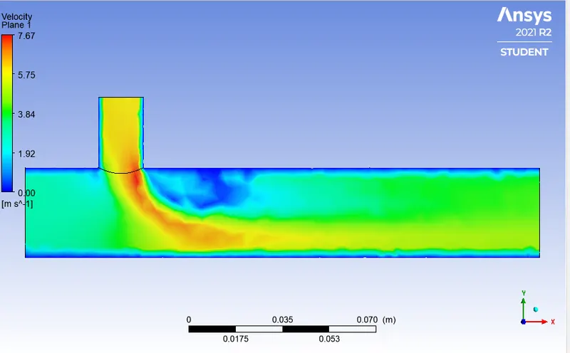
Velocity contour plot

Computational time required for k omega model = 1min 6 sec

The computational time required for k epsilon model is less compared to k omega SST model.

K epsilon is best suited for flow away from the wall, say free surface flow region, whereas k-omega model is best suited for near the wall flow region, where adverse pressure gradient is developed.

So the more suitable model is K epsilon model.

Now we can start doing the 2 cases with different momentum ratios

Case 1-a

Short mixing tee

Hot inlet velocity = 3m/s

Momentum ratio = 2

Cold inlet velocity = 6m/s

The simulation procedure is same as we did the simulation for k epsilon and k omega model.

Results

Convergence plot

Standard deviation of temperature at oulet for each iteration

Area weighted average of temperature at oulet for each iterations

Temperature contour plot

Velocity contour plot

Temperature line plot

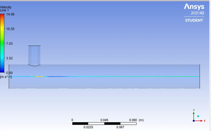
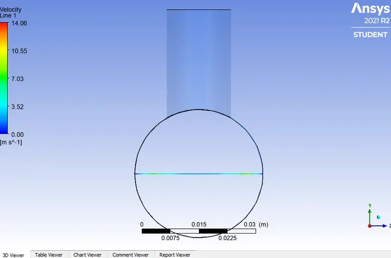
Velocity line plot

Case 1-b

Short mixing tee

Hot inlet velocity = 3m/s

Momentum ratio = 4

Cold inlet velocity = 12m/s

Computational time required = 49 sec

Results

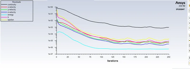
Convergence plot

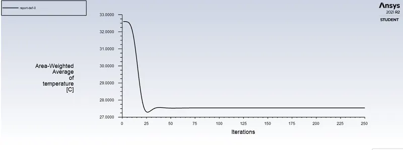
Area weighted average of temperature at oulet for each iterations

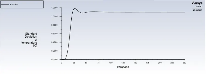
Standard deviation of temperature at oulet for each iteration

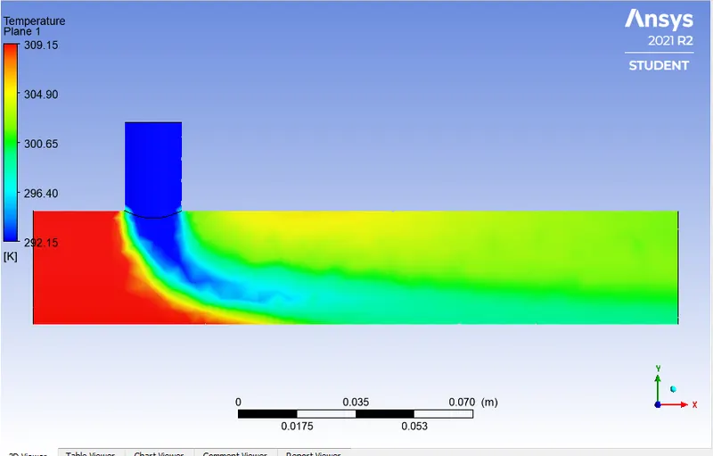
Temperature contour plot

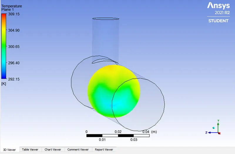
Velocity contour plot

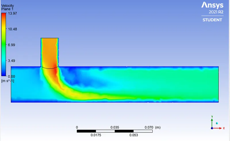
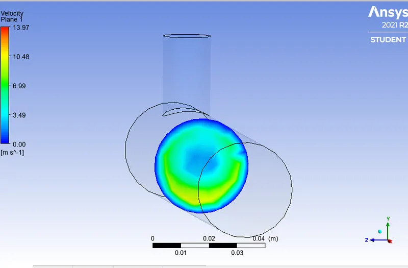
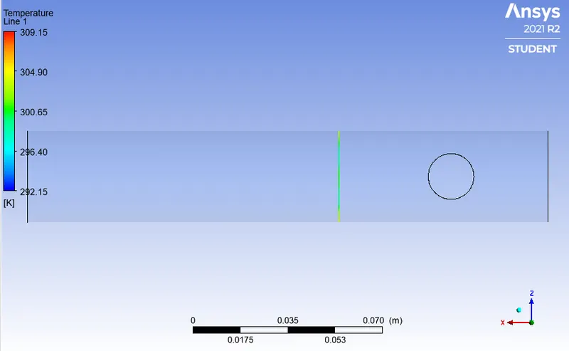
Temperature line plot

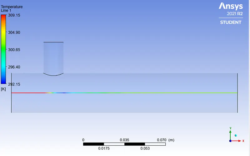
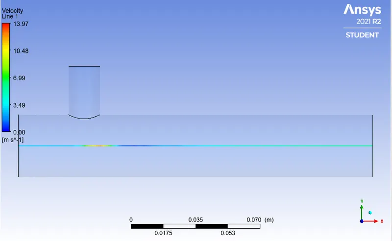
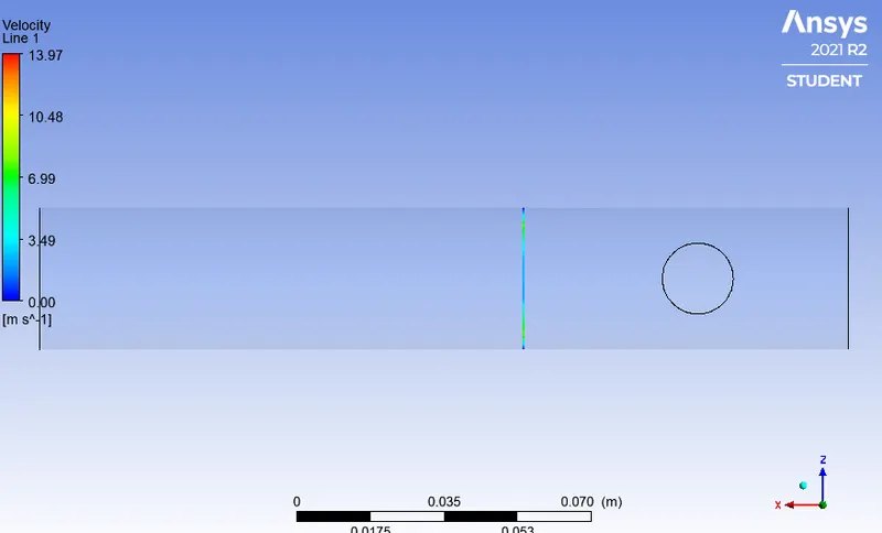
Velocity line plot

Case 2-a

Long mixing tee

Hot inlet velocity = 3m/s

Momentum ratio = 2

Cold inlet velocity = 6m/s

Computational time required = 58 sec

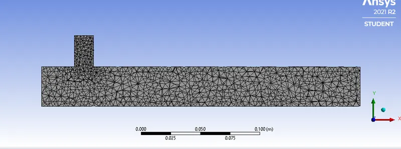
Mesh for long mixing tee

Results

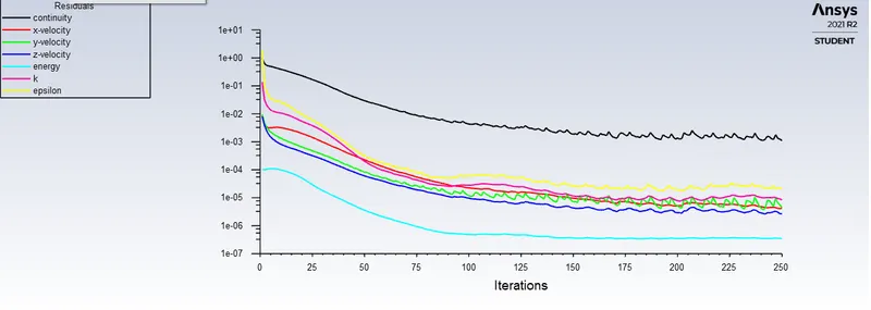
Convergence plot

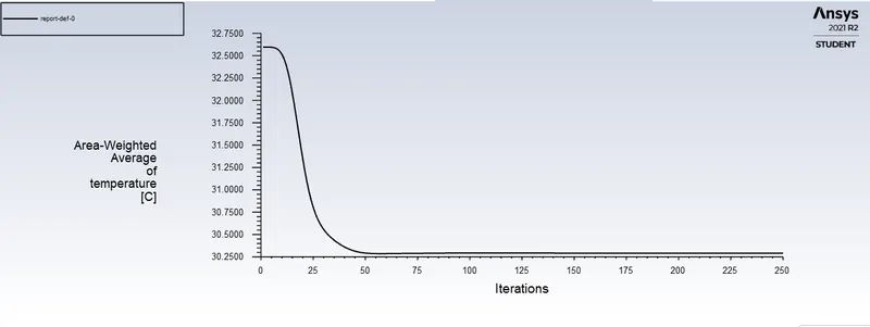
Area weighted average of temperature at oulet for each iterations

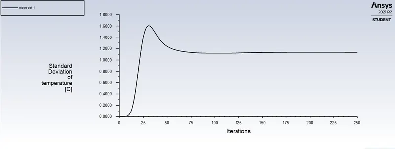
Standard deviation of temperature at oulet for each iteration

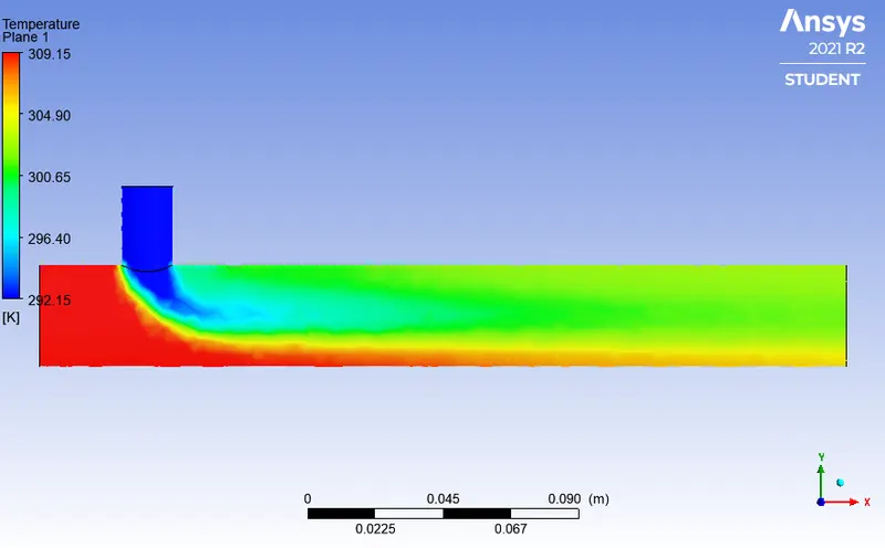
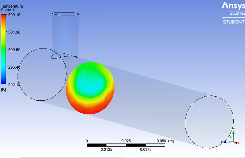
Temperature contour plot

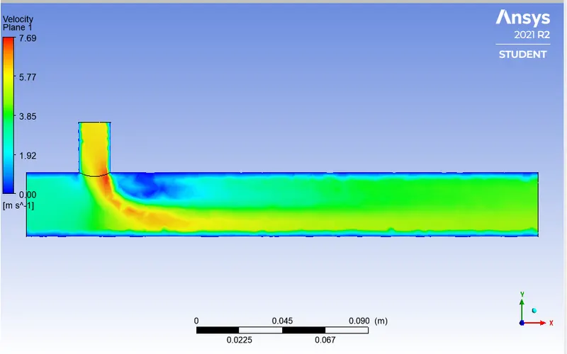
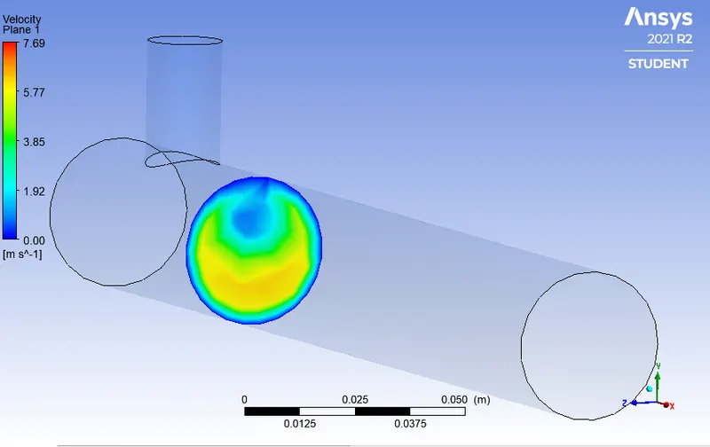
Velocity contour plot

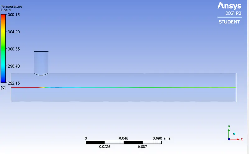
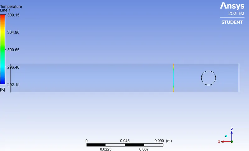
Temperature line plot

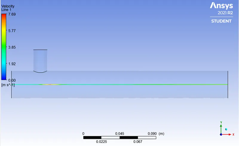
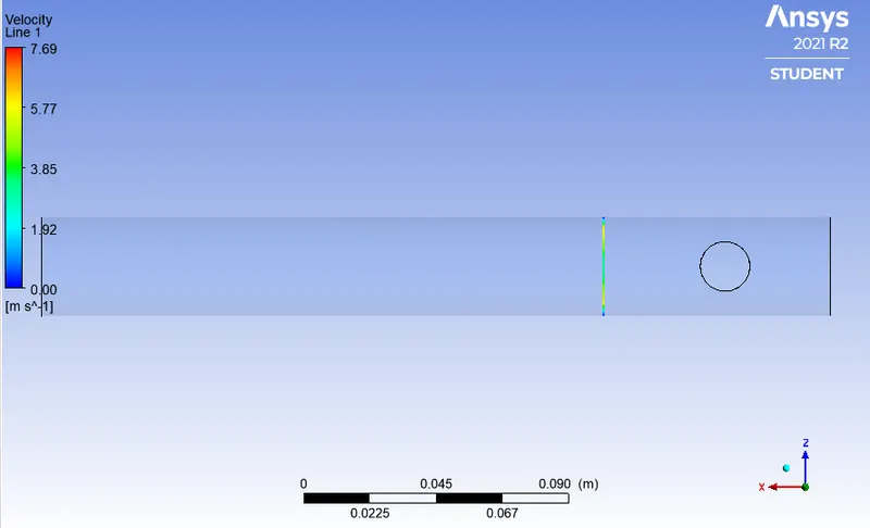
Velocity line plot

Case 2-b

Long mixing tee

Hot inlet velocity = 3m/s

Momentum ratio = 4

Cold inlet velocity = 12m/s

Computational time required = 57 sec

Results

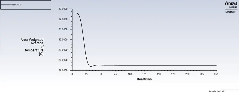
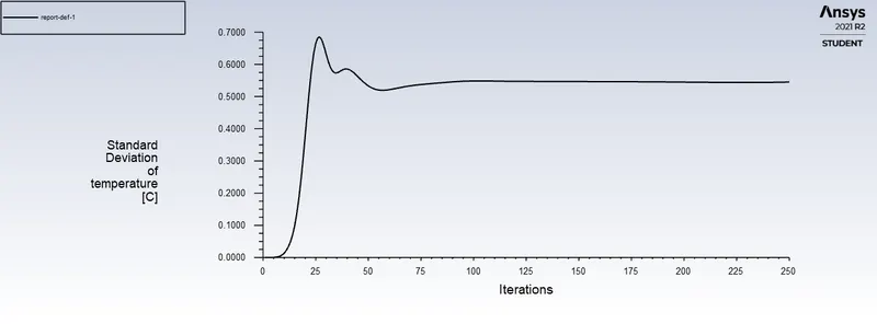
Convergence plot

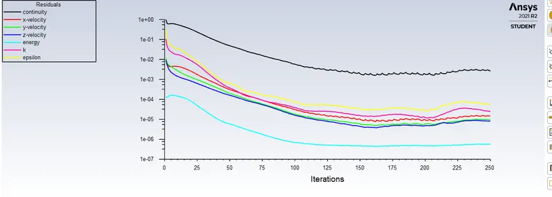
Area weighted average of temperature at oulet for each iterations

Standard deviation of temperature at oulet for each iteration

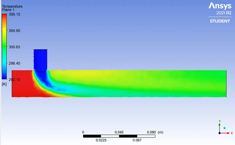
Temperature contour plot

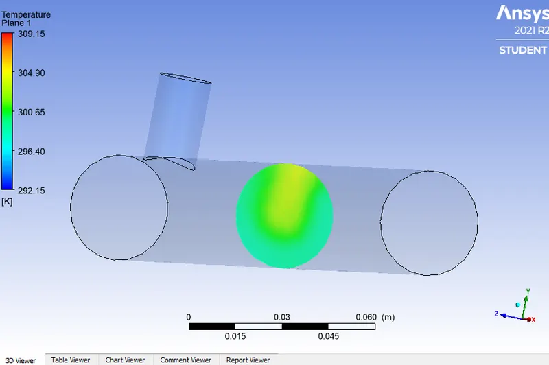
Velocity contour plot

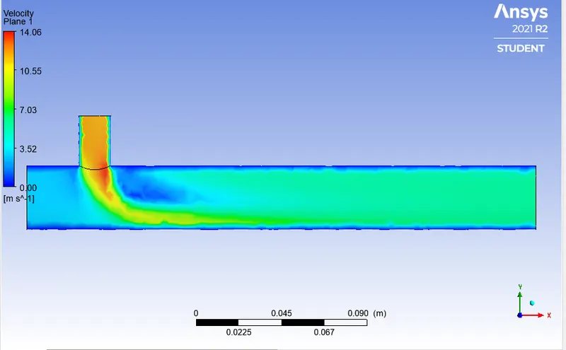
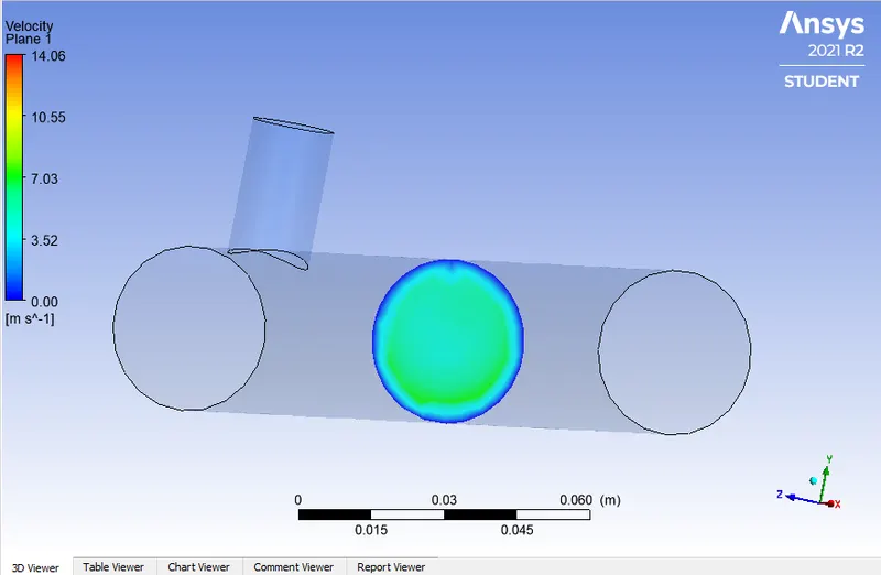
Temperature line plot

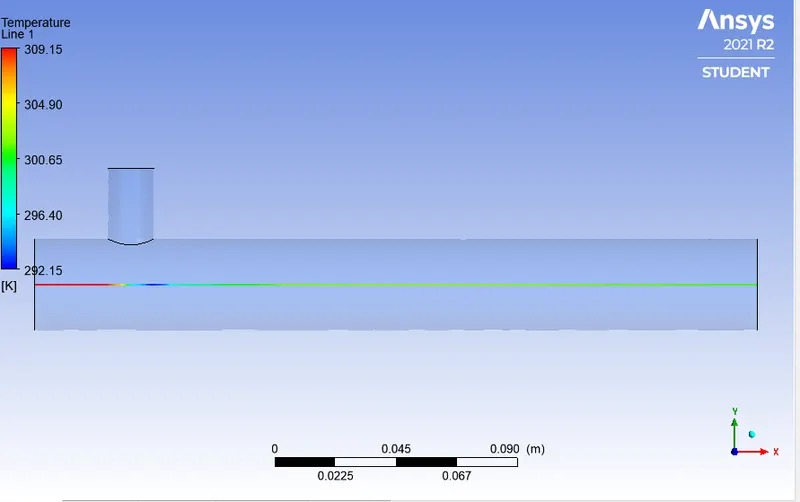
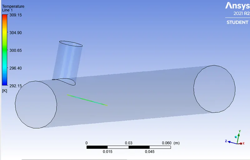
Velocity line plot

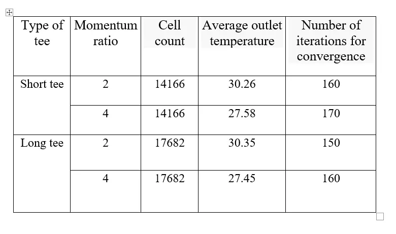
Effect of length and momentum ratio

The outlet temperature is independent of the length of the mixing tee. As the momentum ratio increases the outlet temperature decreases.

Mesh independent study

For this study the short mixing tee is selected with momentum ratio 2.

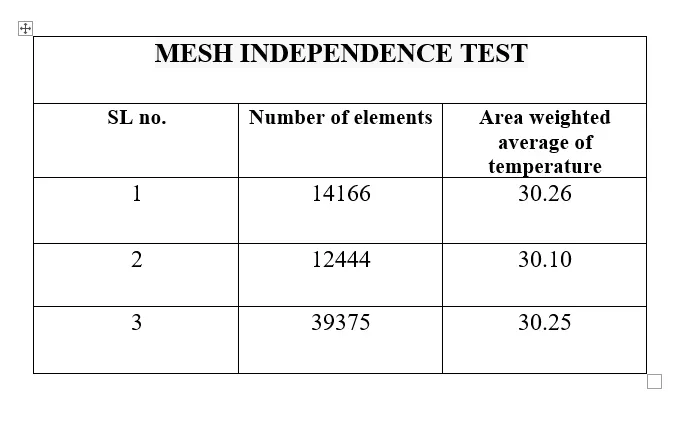
The mesh independency test was conducted for different element sizes. From the above table the mesh independency is proved since there are only small variations in the outlet temperature. The computational time can be reduced by selecting the optimum mesh size without affecting the results.