Week 4 - CHT Analysis on Exhaust port

AIM

To perform CHT Analysis on Exhaust port

OBJECTIVES

1. Give a brief description of why and where a CHT analysis is used.
2. Maintain the y+ value according to the turbulence model and justify the results.
3. Calculate the wall/surface heat transfer coefficient on the internal solid surface & show the velocity & temperature contours in appropriate areas.
4. How would you verify if the HTC predictions from the simulations are right? On what factors does the accuracy of the prediction depend on?

THEORY

Conjugate heat tansfer and Exhaust port

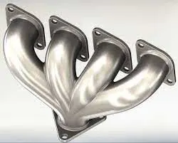
The exhaust manifold is the key component in a 4-stroke IC engine. Exhaust manifold is mounted on the cylinder head of an engine. The exhaust manifold collects exhaust gases from multiple cylinders into one pipe. At the exhaust stroke the exhaust valve open and inlet valve remains closed that time piston starts moving from bottom dead centre to top dead centre sweeps out the burnt gases from the cylinders. These exhaust gases sweeps out from the cylinder and transfer through catalytic converter. The temperature of these of hot gases is near about 800 and pressures is varying about 100 to 500 kpa .This temperature and pressure is experiencing during exhaust stroke. The exhaust manifold made up off gray cast iron is a type of cast iron that has a graphitic microstructure because its ability to tolerate fast and severe temperature changes. When the engine works hard the exhaust manifold can run almost red hot. So we have to investigate the complete behaviour of exhaust manifold experimentally. Only flow or only thermal analysis is not sufficient for engine exhaust system but we have to understand thermal behaviour of structure due to fluid parameter and vice versa by coupling called conjugate heat transfer. The term Conjugate Heat Transfer (CHT) is used to describe processes that involve simultaneous energy exchange between the solid and fluid domains due to interaction between them and is frequently encountered in a variety of engineering applications such as internal combustion engines, turbo-machinery, heat exchangers, etc.

The Conjugate Heat Transfer (CHT) analysis type allows for the simulation of heat transfer between solid and fluid domains by exchanging thermal energy at the interfaces between them. Typical applications of this analysis type exist as, but are not limited to, the simulation of heat exchangers, cooling of electronic equipment, and general-purpose cooling and heating systems. Computational Fluid Dynamics (CFD) and more specifically conjugate heat transfer (CHT) analysis can accurately predict heat transfer by simultaneous solving all the relevant solid and flow field heat transfer processes.

It represents a class of multi-physics problems where fluid flow affects the thermal behaviour of structure, which in turn affects the fluid flow. For conjugate heat transfer analyses, the solid material conduction and the fluid convection are analysed simultaneously. The conductive heat transfer in a solid region is coupled to the convective heat transfer in a neighbouring fluid flow.

Simulation procedure

Open Ansys Workbench, select fluid flow(fluent) and create geometry in spaceclaim.

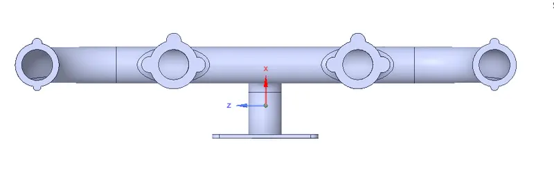
The first step is to extract the fluid volume. But before that we have to remove the dupilcate edges by using extra edges tool.

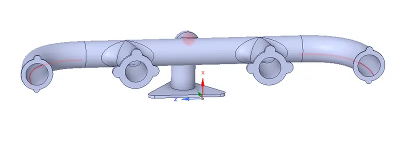
The above figure shows the extra edges in the exhaust port geometry.

Now extraxt the fluid volume, name the two volumes as fluid and solid. Select the two and move into a new component and name it as final geometry. Delete the empty components.

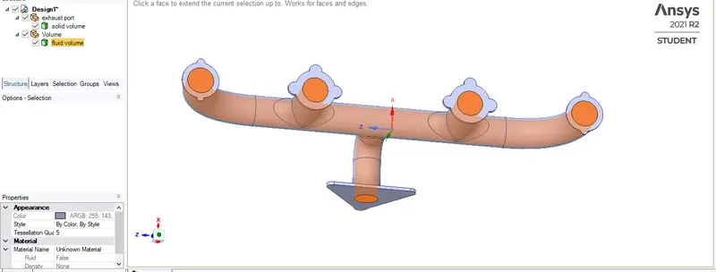
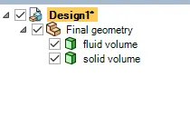
For conjugate heat transfer simulation, the mesh should be conformal. So that the fluid mesh and solid mesh should overlap each other.

For that enable share topology option.

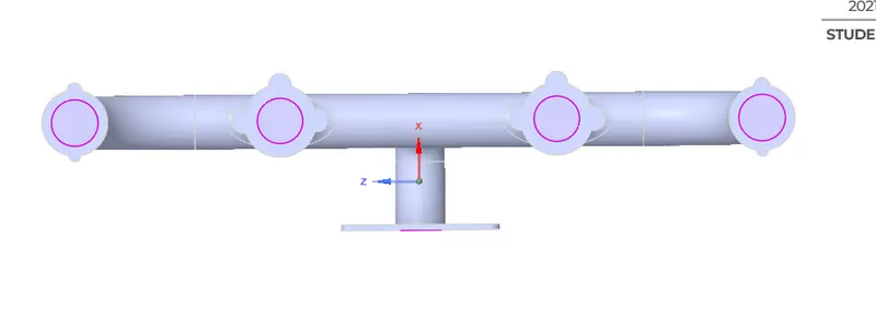
After creating geometry, close spacelaim then the next step is to create the mesh. Before meshing name the boundaries.

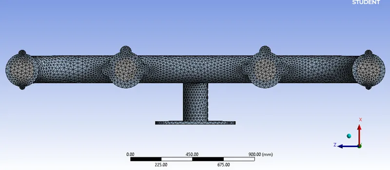
The above figure shows the baseline mesh.

Use body sizing method to refine the mesh and add inflation layers to the internal volume. Find first layer height by choose the y+ value according to the tubulence model. For k-epsilon the target value of y+ should be between 30 and 300.

For this simulation the y+ value = 30

Reference length = 0.1661m, which is the diameter of the inlet

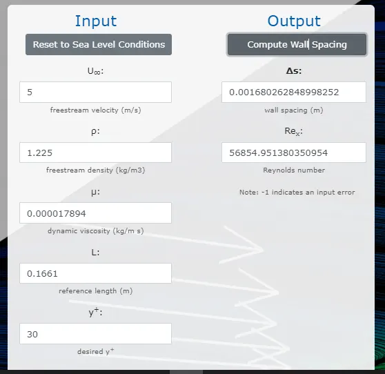
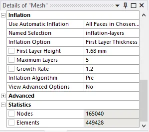
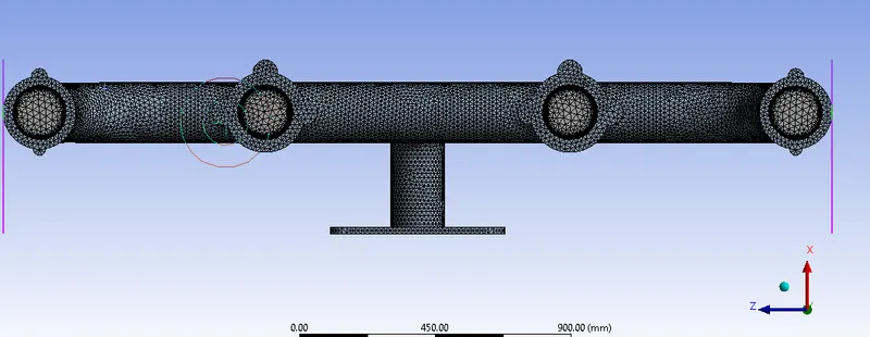
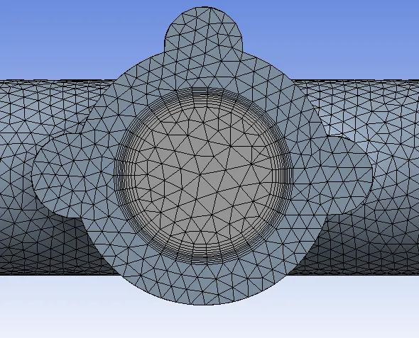
Meshing is complete. Double click on setup to open CFD solver.

Check the mesh quality.

Choose pressure based solver and the simulation is done as steady state simulation.

Enable the energy equation.

Set the viscous model to K-epsilon (standard).

Material : fluid type - air, solid type - aluminium

Set the boundary conditions (inlet velocity = 5m/s, Tempersture = 700k, outlet gauge pressure = 0 Pas, heat transfer coeffecient = 20`W/((m^2*k)`,).

Initialize the solution and run the calculation for 300 iterations.

Results

Residual plot

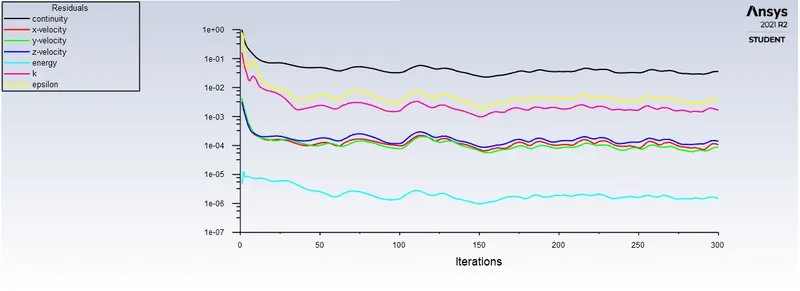
The solution has converged after 200 iterations.

Pressure contour plot

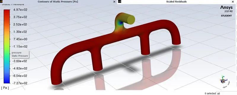
The lowest pressure is in the curve of the outlet port. It is called the back pressure zone of the exhaust manifold. Back pressure usually refers to the pressure exerted on a moving fluid by obstructions against its direction of flow. Back pressure caused by the exhaust system of an automotive engine has a negative effect on engine’s performance as it will restrict the flow rate of the exhaust gasses this will result in reduced engine power.

Temperature contour plot

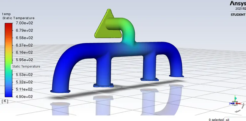
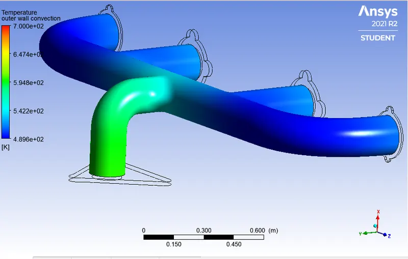
Velocity streamline plot

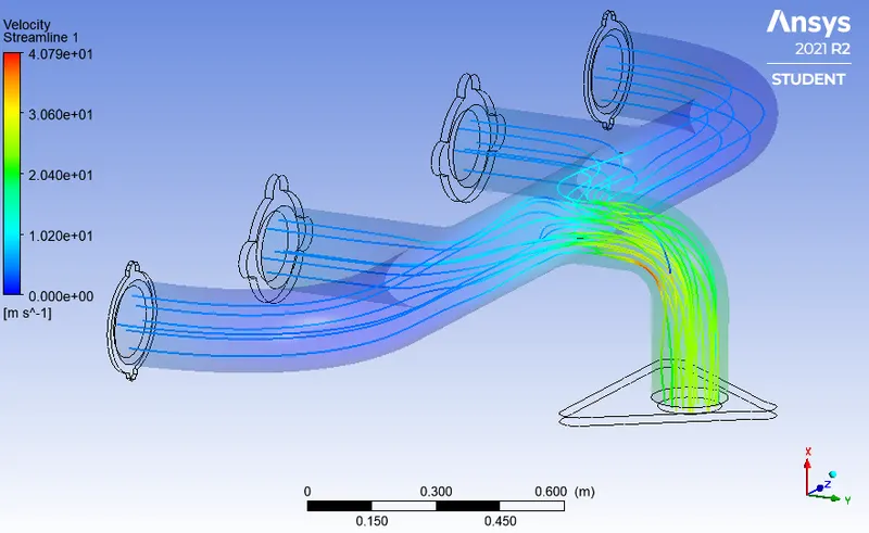
The maximum velocity is in the back pressure zone which is in the vicinity of the exit.

Wall Heat transfer coeffecient plot

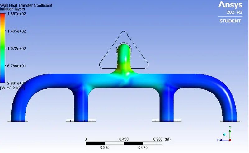
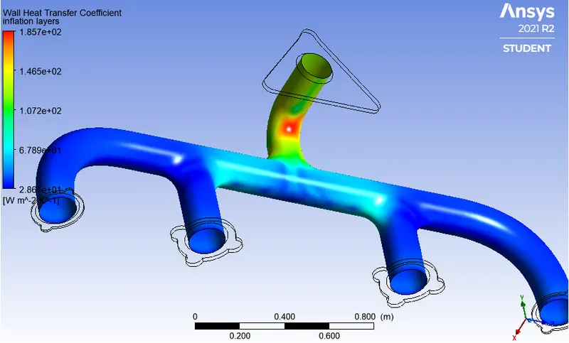
Wall/surface heat transfer coefficient on the internal solid surface

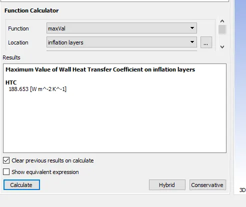
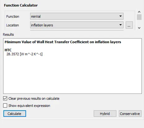
The HTC predictions from the simulations can be verified by comparing it with the numerical results.

To calculate the HTC value numerically we have to find the Nusselt number. The Nusselt number is the ratio of convective to conductive heat transfer across a boundary.

To determine Nusselt number, the Dittus-Boelter equation can be used.

where:

D is the inside diameter of the circular duct
Pr is the Prandtl number
n=0.4 for the fluid being heated, and n=0.3 for the fluid being cooled.

From the Nusselt number value we can find the value of HTC

`N_u = (h*L)/k`

where h is the convective heat transfer coefficient of the flow, L is the characteristic length, k is the thermal conductivity of the fluid.

The accuracy of the prediction depends upon:

• Better mesh refinement
• Proper selection of y+ value according to the turbulence model

CONCLUSION

• CHT analysis was conducted on exhaust port.
• Wall heat transfer coeffecient is highest on the back pressure zone which is very close to the outlet. In this region the velocity is also maximum.
• Better results can be obtained by refining the mesh and by choosing proper y+ values according to the turbulence model.

Reference : Liao, Liang, et al. "Numerical study of Conjugate heat transfer in a BIPV-thermal system." International Solar Energy Conference. Vol. 47373. 2005.