Week 3.5 - Deriving 4th order approximation of a 2nd order derivative using Taylor Table method

AIM

Derive the following 4th order approximations of the second-order derivative.

1. Central difference

2. Skewed right-sided difference

3. Skewed left-sided difference

After deriving these schemes, prove that your skewed schemes are fourth-order accurate i.e the thumb rule

Once you have done this, write a program in Matlab to evaluate the second-order derivative of the analytical function exp(x)*cos(x) and compare it with the 3 numerical approximations that you have derived.

Provide a plot that compares the absolute error between the above-mentioned schemes

In your own words, describe why a skewed scheme is useful? What can a skewed scheme do that a CD scheme cannot?

1. Deriving the 4th order approximation of the second-order derivative by central difference method

No. of nodes,N = P+Q-1 = 4+2-1 = 5

`(deltax^2)*((del^2f)/(delx^2)) = a*f(i-2)+b*f(i-1)+c*f(i)+d*f(i+1)+e*f(i+2)`

the TAYLOR's TABLE for the above equation,

	`f(i)`	`deltax*f'(i)`	`deltax^2*f''(i)`	`deltax^3*f'''(i)`	`deltax^4*f^4(i)`	`deltax^5*f^5(i)`	`deltax^6*f^6(i)`
`a*f(i-2)`	a	-2a	2a	`-4/3a`	`2/3a`	`-4/15a`	`4a/45`
`b*f(i-1)`	b	-b	`b/2`	`-b/6`	`b/24`	`-b/120`	`b/720`
`c*f(i)`	c	0	0	0	0	0	0
`d*f(i+1)`	d	d	`d/2`	`d/6`	`d/24`	`d/120`	d/720
`e*f(i+2)`	e	2e	2e	`4/3e`	`2/3e`	`4/15e`	`4e/45`
	0	0	1	0	0	0	don't know

Now, we get

`a+b+c+d+e=0`

`-2a-b+d+2e=0`

`2a+b/2+d/2+2e=1`

`-4/3a-b/6+d/6+4/3e=0`

`2/3a+b/24+d/24+2/3e=0`

converting into matrix form and solving in matlab

clear all 
close all
clc

%to solve the matrix equation
A=[1 1 1 1 1;-2 -1 0 1 2;2 1/2 0 1/2 2;-4/3 -1/6 0 1/6 4/3;2/3 1/24 0 1/24 2/3];
B=[0;0;1;0;0];
X=linsolve(A,B)

Output

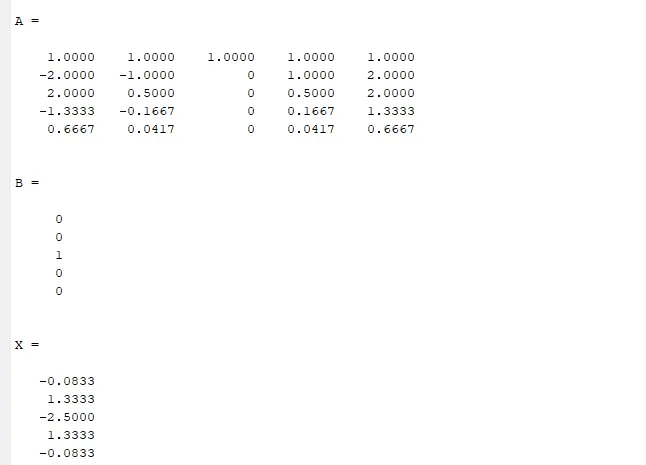
`(deltax^2)*((del^2f)/(delx^2)) = a*f(i-2)+b*f(i-1)+c*f(i)+d*f(i+1)+e*f(i+2)`

`(deltax^2)*((del^2f)/(delx^2)) = (a+b+c+d+e)f(x)+(-2a-b+d+2e)(deltax)f'(x)+(2a+b/2+d/2+2e)(deltax^2)f''(x)+(-4a/3-b/6+d/6+4e/3)(deltax^3)f'''(x)+(2a/3+b/24+d/24+2e/3)(deltax^4)f^4(x)+(-4a/15+b/120+d/120+4e/15)(deltax^5)f^5(x)+(4a/45+b/720+d/720+4e/45)(deltax^6)f^6(x)`

substituting the coeffecients we get

`((del^2f)/(delx^2))= ((-0.0833)f(i-2)+(1.3333)f(i-1)+(-2.5)f(i)+(1.3333)f(i+1)+(-0.0833)f(i+2))/(deltax^2)`

2. Deriving the 4th order approximation of the second-order derivative by skewed right-sided difference method

No. of nodes = P+Q = 4+2 = 6

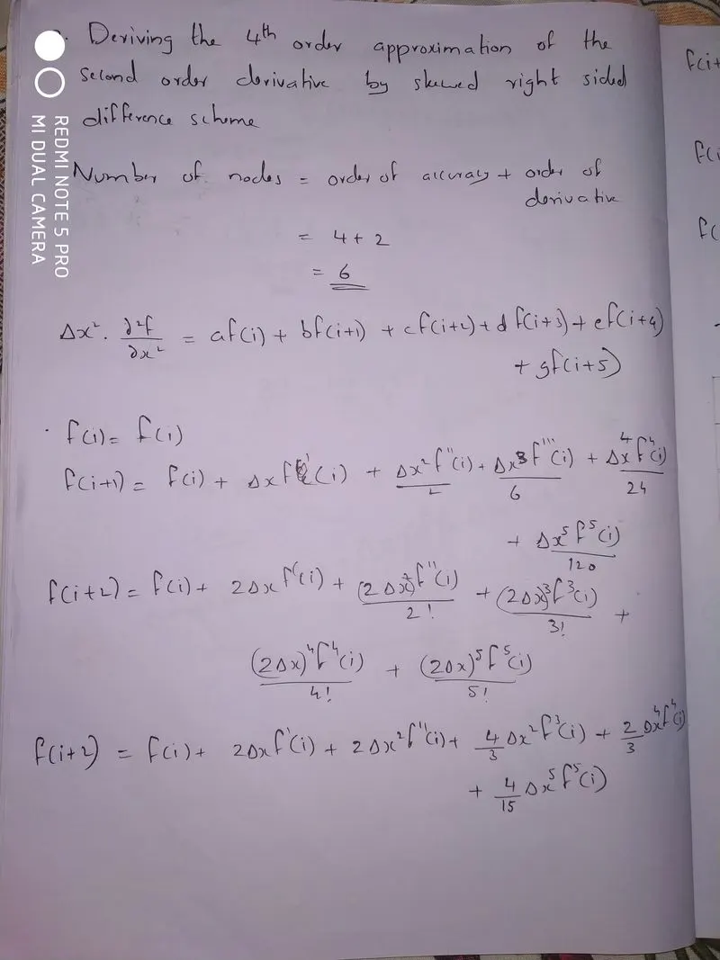
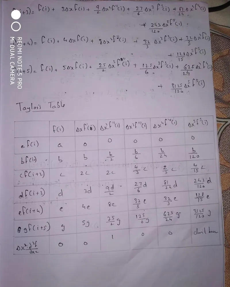
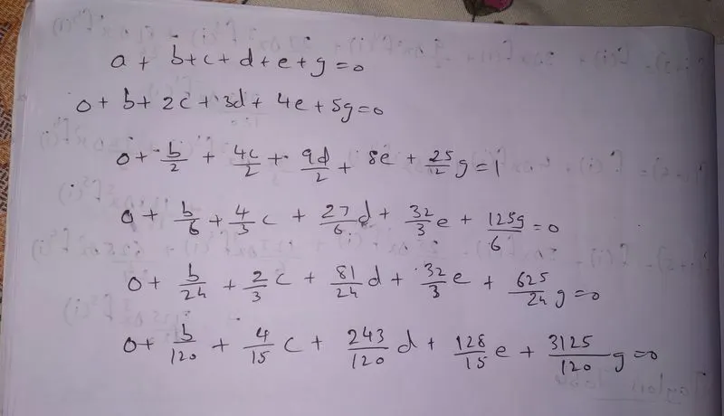
converting into matrix form and solving in matlab;

clear all 
close all
clc

%to solve the matrix equation
A=[1 1 1 1 1 1;0 1 2 3 4 5;0 1/2 2 9/2 8 25/2;0 1/6 4/3 27/6 32/3 125/6;0 1/24 2/3 81/24 32/3 625/24;0 1/120 4/15 243/120 128/15 3125/120] 
B=[0;0;1;0;0;0]
X=linsolve(A,B)

ouput

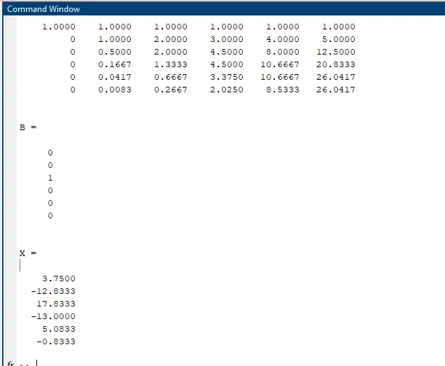
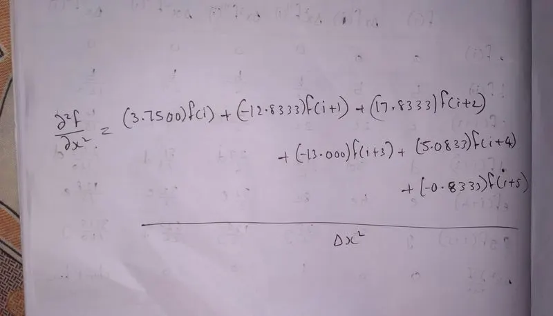
substituting the coeffecients in the equation, we get

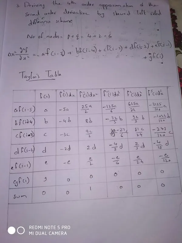
3. Deriving the 4th order approximation of the second-order derivative by skewed left-sided difference method

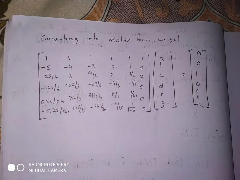
converting into matrix form

code to solve the matrix equation

clear all 
close all
clc

%to solve the matrix equation
A=[1 1 1 1 1 1;-5 -4 -3 -2 -1 0;25/2 8 9/2 2 1/2 0;-125/6 -32/3 -27/6 -4/3 -1/6 0;625/24 32/3 81/24 2/3 1/24 0;-3125/120 -128/15 -243/120 -4/15 -1/120 0] 
B=[0;0;1;0;0;0]
X=linsolve(A,B)

output

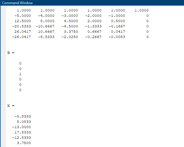
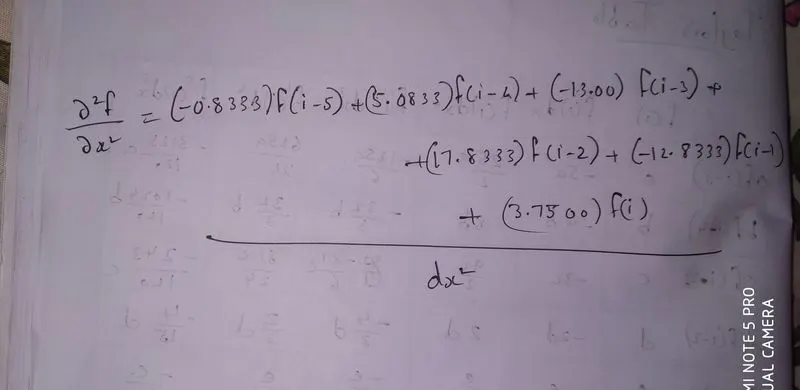
substituting the coeffecients we get

MAIN CODE

clear all
close all
clc

%assign value to x
x=pi/3;

%range of dx
dx=linspace(pi/40,pi/4000,20);

for i=1:length(dx)
    central_differencing(i)=central_difference(x,dx(i));
    right_sidedskew(i)=Skewed_right_sided_difference(x,dx(i));
    left_sidedskew(i)=Skewed_leftsided_difference(x,dx(i));
end

%plot the graph

figure(1)
loglog(dx,central_differencing,'r');
hold on
loglog(dx,right_sidedskew,'g');
hold on
loglog(dx,left_sidedskew,'b');
xlabel('dx');
ylabel('error');
legend('central difference','Skewed right-sided difference','Skewed left-sided difference','location','best')
title('Error Comparison');

Function code

function error_cds = central_difference(x,dx)
%analytical function f(x) = exp(x)*cos(x)
%second order derivative,f''(x)=-2*exp(x)*sin(x)
analytical_derivative = -2*exp(x)*sin(x);

%central differencing
central_differencing = (((-0.08333333333333333333333333333333)*(exp(x-(2*dx)))*(cos(x-(2*dx))))+((1.3333333333333333333333333)*(exp(x-dx))*(cos(x-dx)))+((-2.5000)*(exp(x)*cos(x)))+((1.333333333333333333333333333333)*(exp(x+dx))*(cos(x+dx)))+((-0.08333333333333333333333333333)*(exp(x+(2*dx)))*(cos(x+(2*dx)))))/(dx^2)

%error
error_cds= abs(central_differencing-analytical_derivative);
end

function error_rightsds =Skewed_right_sided_difference(x,dx)
%analytical function f(x) = exp(x)*cos(x)
%second order derivative,f''(x)=-2*exp(x)*sin(x)
analytical_derivative = -2*exp(x)*sin(x);

%Skewed right-sided difference
Skewed_rightsided_difference = (((3.7500)*(exp(x))*(cos(x)))+((-12.8333333333333333333333333333333)*(exp(x+dx))*(cos(x+dx)))+((17.833333333333333333333333333333)*(exp(x+(2*dx))*cos(x+(2*dx))))+((-13.000)*(exp(x+(3*dx)))*(cos(x+(3*dx))))+((5.0833333333333333333333333)*(exp(x+(4*dx)))*(cos(x+(4*dx))))+((-0.83333333333333333333333)*(exp(x+(5*dx)))*(cos(x+(5*dx)))))/(dx^2)

%error
error_rightsds= abs(Skewed_rightsided_difference-analytical_derivative);
end

function error_leftsds =Skewed_leftsided_difference(x,dx)
%analytical function f(x) = exp(x)*cos(x)
%second order derivative,f''(x)=-2*exp(x)*sin(x)
analytical_derivative = -2*exp(x)*sin(x);

%Skewed right-sided difference
%Skewed_leftsided_difference = (((-0.833333333333333333333333)*((exp(x-(5*dx)))*(cos(x-(5*dx)))))+((5.08333333333333333333333333333333)*((exp(x-(4*dx)))*(cos(x-(4*dx)))))+((-13.000)*((exp(x-(3*dx)))*cos(x-(3*dx)))))+((17.833333333333333333333333333333)*((exp(x-(2*dx)))*(cos(x-(2*dx)))))+((-12.833333333333333333333333333333)*((exp(x-dx))*(cos(x-dx))))+((3.7500)*((exp(x))*(cos(x))))/(dx^2)
Skewed_leftsided_difference =(((3.7500)*(exp(x))*(cos(x)))+((-12.8333333333333333333333333333333)*(exp(x-dx))*(cos(x-dx)))+((17.833333333333333333333333333333)*(exp(x-(2*dx))*cos(x-(2*dx))))+((-13.000)*(exp(x-(3*dx)))*(cos(x-(3*dx))))+((5.0833333333333333333333333)*(exp(x-(4*dx)))*(cos(x-(4*dx))))+((-0.83333333333333333333333)*(exp(x-(5*dx)))*(cos(x-(5*dx)))))/(dx^2)
%error
error_leftsds= abs(Skewed_leftsided_difference-analytical_derivative);
end

Results

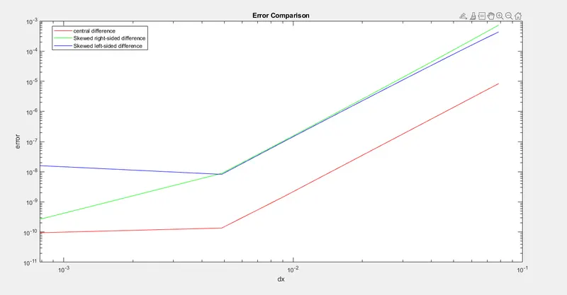
The graph shows that the central scheme is more accurate than the skewed differencing scheme. The graph also shows that when the value of dx is very small the curves becomes unstable due to the combination of various errors such as truncation error, round off error etc.

A skewed scheme is useful when the information of both sides of the nodes are not sufficient. CDS requires information on both sides of the node. Skewed schemes requires information on only one side.