Week 7 - Simulation of a 1D Super-sonic nozzle flow simulation using Macormack Method
AIM
In this challenge you are going to simulate the isentropic flow through a quasi 1D subsonic-supersonic nozzle. You will derive both the conservation and non-conservation forms of the governing equations and sovle them using the MacCormack's technique. You need to determine the steady-state temperature distribution for the flow-field variables and investigate the difference between the two forms of governing equations by comparing their solutions.
You need to show the following plots inside your report
1. Steady-state distribution of primitive variables inside the nozzle
2. Time-wise variation of the primitive variables
3. Variation of Mass flow rate distribution inside the nozzle at different time steps during the time-marching process
4. Comparison of Normalized mass flow rate distributions of both forms
THEORY
Subsonic-supersonic isentropic flow
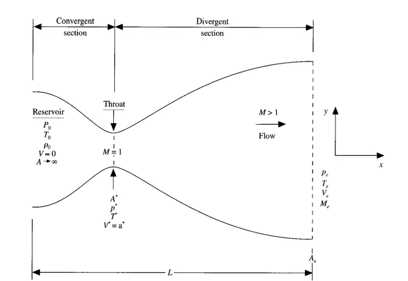
Consider a steady,isentropic flow through a covergent divergent nozzle as shown in the above figure. The flow at the inlet to the nozzle comes from a reservoir where the pressure and temperature are denoted by P0 and T0 respectively. The cross sectional area of the reservoir is large hence the velocity is small. The flow expands isentropically to supersonic speeds at the nozzle exit where the pressure, temperature, veloxity and mach number are denoted by Pe, Te, Ve, Me respectively. The flow is locally subsonic at the convergent section of the nozzle, sonic at the throat and supersonic at the divergent section. The area of the sonic throat is denoted by A*.
We assume that at a given section where the cross sectional area is A, the flow properties are unifrom across that section. Hence although the area of the nozzle changes as a function of distance along the nozzle x, therefore in reality the flow field is two dimensional, we make the assumption that the flow properties vary only along with x. Such flow is defined as quasi-one-dimensional flow.
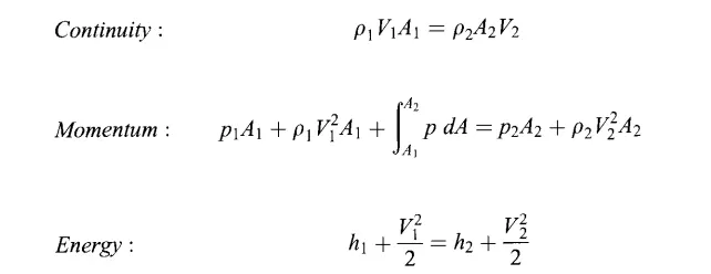
The governing continuity, momentum and energy equations for quasi-one-dimensional steady isentropic flow is given below
The Mach number variation through the nozzle is governed exclusively by the area ratio through the relation

Governing equations in the Non-conservational form (non-dimensional variables)
Continuity eqn
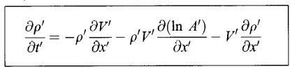
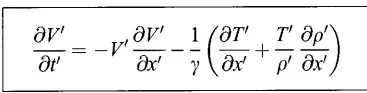
Momentum eqn
Energy eqn

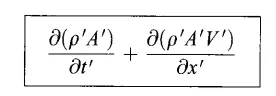
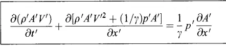
Governing equations in the Conservational form (non-dimensional variables)
Continuity eqn
Momentum eqn
Energy eqn

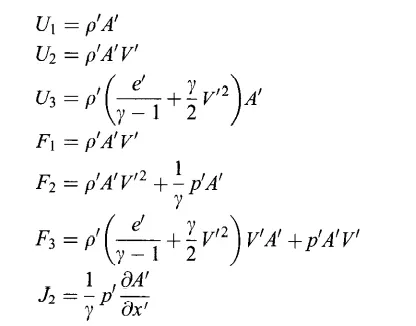
The source vector U, the flux vector F and the source term J are as follows:
Then the governing eqns in the conservation form can be written as
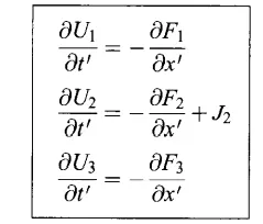
Here the dependant variables are not primitive variables, hence the numerical solution will give values for solution vectors. Then values for primitive variables should be decoded from them.
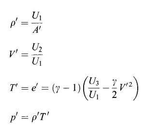
Calculation of time step
`Deltat = C(Deltax)/(a+V`
where, C = courant number
a = local velocity of sound
V = local flow velocity
The MacCormack explicit technique is used to solve the problem.
MacCormack method - In CFD, the MacCormack method is a widely used discretization scheme for the numerical solution of hyperbolic partial differential equations. This second-order finite difference method was introduced by Robert W. MacCormack in 1969. The MacCormack method is elegant and easy to understand and program. The MacCormack method is a two-steps method (predictor-corrector) of second-order accuracy in both space and time and this method is commonly utilized in the resolution of compressible fluids problems.
In the time marching approach, we know the flow field variables at time t, and we use the difference equations to solve explicitly for the variables at time `t+Deltat`.
Main code
clear all
close all
clc

%inputs
n=31;
x=linspace(0,3,n);

dx=x(2)-x(1);
nt=1400;

% t= temperature;
% v = velocity;
% g = gamma
% a = area
% C = 0.5(courant number)
%rho = density
%M= mach number
%m=mass flow rate
%n=node;


%area
a= 1+2.2*(x-1.5).^2;

%non-conservative form
[rho_nc,v_nc,t_nc,M_nc,m_nc,p_nc,t_throat,p_throat,M_throat,rho_throat] = non_conservative_form(n,x,dx);


%conservative form
[rho_c,v_c,t_c,m_c,t_cthroat,p_cthroat,rho_cthroat,M_cthroat,M_c,p_c] = conservative_form(n,x,dx);


%plotting
%non-conservative form
%Steady-state distribution of primitive variables inside the nozzle
figure(3)
subplot(4,1,1)
plot(x,p_nc);
title('Distribution of primitive variables inside the nozzle(Non-conservative form)');
xlabel('Distance');
ylabel('Pressure');
hold on

subplot(4,1,2)
plot(x,M_nc);

xlabel('Distance');
ylabel('Mach number');
hold on

subplot(4,1,3)
plot(x,rho_nc);
xlabel('Distance');
ylabel('Density');
hold on

subplot(4,1,4)
plot(x,t_nc);
xlabel('Distance');
ylabel('Temperature');
hold on


%Time-wise variation of the primitive variables
%Non conservation form
figure(7)
subplot(4,1,1)
plot(rho_throat);
title('Time-wise variation of the primitive variables (Non-Conservation form)');
xlabel('Number of timesteps');
ylabel('Density');
hold on

subplot(4,1,2)
plot(t_throat);
xlabel('Number of timesteps');
ylabel('Temperature');
hold on

subplot(4,1,3)
plot(p_throat);
xlabel('Number of timesteps');
ylabel('Pressure');
hold on

subplot(4,1,4)
plot(M_throat);
xlabel('Number of timesteps');
ylabel('Mach number');
hold on


%conservative form
%Steady-state distribution of primitive variables inside the nozzle
figure(5)
subplot(4,1,1)
plot(x,p_c);
title('Distribution of primitive variables inside the nozzle (Conservative form)');
xlabel('Distance');
ylabel('Pressure');
hold on

subplot(4,1,2)
plot(x,M_c);

xlabel('Distance');
ylabel('Mach number');
hold on

subplot(4,1,3)
plot(x,rho_c);
xlabel('Distance');
ylabel('Density');
hold on

subplot(4,1,4)
plot(x,t_c);
xlabel('Distance');
ylabel('Temperature');
hold on

%Time-wise variation of the primitive variables
% conservation form
figure(8)
subplot(4,1,1)
plot(rho_cthroat);
title('Time-wise variation of the primitive variables (Conservation form)');
xlabel('Number of timesteps');
ylabel('Density');
hold on

subplot(4,1,2)
plot(p_cthroat);
xlabel('Number of timesteps');
ylabel('Pressure');
hold on

subplot(4,1,3)
plot(M_cthroat);
xlabel('Number of timesteps');
ylabel('Mach number');
hold on

subplot(4,1,4)
plot(t_cthroat);
xlabel('Number of timesteps');
ylabel('Temperature');
hold on


figure(6)
plot(x,m_nc)
hold on
plot(x,m_c)
hold on
line([0 3],[0.579 0.579])
xlabel('x/L');
ylabel('Mass flow rate');
title('Steady state mass flow variations');
legend('Non-conservation form','Conservation form','Exact analytical solution');
Function Code for Non-conservation form
%function code- non conservative form
function [rho_nc,v_nc,t_nc,M_nc,m_nc,p_nc,t_throat,p_throat,M_throat,rho_throat] = non_conservative_form(n,x,dx)


%caclulate initial profiles
rho_nc= 1-0.3146*x;
t_nc=1-0.2314*x; %temperature
v_nc= (0.1+1.09*x).*t_nc.^0.5;


gamma =1.4;

%area
a= 1+2.2*(x-1.5).^2;

%timesteps
nt=1400;

C = 0.5; %courant number


%outer time loop
for k = 1:nt

    rho_old = rho_nc;
    t_old = t_nc;
    v_old = v_nc;

   dt = min(C.*dx./(sqrt(t_nc)+ v_nc)) ;

%predictor step
for j = 2:n-1

    dvdx = (v_nc(j+1)-v_nc(j))/dx;
    drhodx = (rho_nc(j+1)-rho_nc(j))/dx;
    dtdx = (t_nc(j+1)-t_nc(j))/dx;
    dlogadx = (log(a(j+1))-log(a(j)))/dx;

    %continuity equation
    drhodt_p(j) = -rho_nc(j)*dvdx-rho_nc(j)*v_nc(j)*dlogadx-v_nc(j)*drhodx;

    %momentum equation
    dvdt_p(j) = -v_nc(j)*dvdx-(1/gamma)*(dtdx+(t_nc(j)/rho_nc(j))*drhodx);

    %energy equation
    dtdt_p(j) = -v_nc(j)*dtdx-(gamma-1)*t_nc(j)*(dvdx+v_nc(j)*dlogadx);

    %solution update

    rho_nc(j) = rho_nc(j) + drhodt_p(j)*dt;
    v_nc(j) = v_nc(j) + dvdt_p(j)*dt;
    t_nc(j) = t_nc(j) + dtdt_p(j)*dt;


end

%corrector method

for j = 2:n-1

    dvdx = (v_nc(j)-v_nc(j-1))/dx;
    drhodx = (rho_nc(j)-rho_nc(j-1))/dx;
    dtdx = (t_nc(j)-t_nc(j-1))/dx;
    dlogadx = (log(a(j))-log(a(j-1)))/dx;

    %continuity equation
    drhodt_c(j) = -rho_nc(j)*dvdx-rho_nc(j)*v_nc(j)*dlogadx-v_nc(j)*drhodx;

    %momentum equation
    dvdt_c(j) = -v_nc(j)*dvdx-(1/gamma)*(dtdx+(t_nc(j)/rho_nc(j))*drhodx);

    %energy equation
    dtdt_c(j) = -v_nc(j)*dtdx-(gamma-1)*t_nc(j)*(dvdx+v_nc(j)*dlogadx);


end


%compute the average time derivative

drhodt_avg = 0.5*(drhodt_p + drhodt_c);
dvdt_avg = 0.5*(dvdt_p + dvdt_c);
dtdt_avg = 0.5*(dtdt_p + dtdt_c);

%final solution update

for i = 2:n-1
    rho_nc(i) = rho_old(i) + drhodt_avg(i)*dt;
    v_nc(i) = v_old(i) + dvdt_avg(i)*dt;
    t_nc(i) = t_old(i) + dtdt_avg(i)*dt;
end


%Apply the boundary conditions
%inlet
v_nc(1) = 2*v_nc(2)-v_nc(3);

%outlet
rho_nc(n) = 2*rho_nc(n-1)-rho_nc(n-2);
v_nc(n) = 2*v_nc(n-1)-v_nc(n-2);
t_nc(n) = 2*t_nc(n-1)-t_nc(n-2);


M_nc = v_nc./sqrt(t_nc); %Mach number
p_nc = rho_nc.*t_nc; %pressure
m_nc = rho_nc.*a.*v_nc; %massflowrate

throat=16;
t_throat(k)=t_nc(throat);
M_throat(k)=M_nc(throat);
p_throat(k)=p_nc(throat);
rho_throat(k)=rho_nc(throat);


%plotting mass flow rate at different timesteps
figure(1)
if k == 1
    plot(x,m_nc,'b--','linewidth',1.75);
    hold on
elseif k == 50
    plot(x,m_nc,'m','linewidth',1.75)
    hold on
elseif k == 100
      plot(x,m_nc,'r','linewidth',1.75)
       hold on
elseif k == 150
     plot(x,m_nc,'g','linewidth',1.75)
      hold on
elseif k == 200
     plot(x,m_nc,'y','linewidth',1.75)
      hold on
     elseif k == 700
     plot(x,m_nc,'k','linewidth',1.75)


     xlabel('Non-dimensional distance throught the nozzle');
     ylabel('Non-dimensional mass flow rate');
     title('Non-dimensional mass flow rate (non conservative form)');
     legend({'0 timesteps','50 timesteps','100 timesteps','150 timesteps','200 timesteps','700 timesteps'})
end


end

end
Function Code for Conservation form
%function code for conservative form

function [rho_c,v_c,t_c,m_c,t_cthroat,p_cthroat,rho_cthroat,M_cthroat,M_c,p_c] = conservative_form(n,x,dx)


g =1.4;%gamma

C = 0.5; %courant number


%timesteps
nt=1400;

%initial conditions

for i= 1:length(x)
    if (x(i)>=0)&&(x(i)<=0.5)
        rho_c(i)=1;
        t_c(i)=1;

    elseif (x(i)>=0.5)&&(x(i)<=1.5)
        rho_c(i) = 1-0.336.*(x(i)-0.5);
        t_c(i) = 1-0.167.*(x(i)-0.5);

    elseif (x(i)>=1.5)&&(x(i)<=3.5)
        rho_c(i) = 0.634-0.3879.*(x(i)-1.5);
        t_c(i) = 0.833-0.3507.*(x(i)-1.5);
    end
end

%area
a= 1+2.2*(x-1.5).^2;


%solution vectors


U1 = rho_c.*a;

%velocity
v_c=(0.59)./(rho_c.*a);

U2 = rho_c.*a.*v_c;
U3 = rho_c.*((t_c./(g-1))+((g/2).*v_c.^2)).*a;


for k = 1:nt

    U1_old = U1;
    U2_old = U2;
    U3_old = U3;

    dt = min(C.*dx./(sqrt(t_c)+ v_c));

  %initialization of flux
   F1 = U2;
    F2 = ((U2.^2)./U1)+((g-1)/g)*(U3-(g/2)*((U2.^2)./U1));
    F3 = ((g.*U2.*U3)./U1)-((g*(g-1))/2).*((U2.^3)./(U1.^2));


%predictor

    for j=2:n-1
        J(j) = (1/g)*rho_c(j)*t_c(j)*((a(j+1)-a(j))/dx);

          dU1dt_p(j) = -((F1(j+1)-(F1(j)))/dx);
          dU2dt_p(j) = -((F2(j+1)-(F2(j)))/dx)+J(j);
          dU3dt_p(j) = -((F3(j+1)-(F3(j)))/dx);

          %obtaining intermediate solution

          U1(j) = U1_old(j) + (dU1dt_p(j))*dt;
          U2(j) = U2_old(j) + (dU2dt_p(j))*dt;
          U3(j) = U3_old(j) + (dU3dt_p(j))*dt;

    end

         %computing primitive variables
         rho_c = U1./a;
         v_c = U2./U1;

         t_c = (g-1).*((U3./U1)-((g/2).*((U2./U1).^2)));


      %recomputing from the predictor updated values of U1,U2,U3
          F1 = U2;
          F2 = ((U2.^2)./U1)+((g-1)/g).*(U3-(g/2)*((U2.^2)./U1));
          F3 = ((g.*U2.*U3)./U1)-((g*(g-1))/2).*((U2.^3)./(U1.^2));


         %corrector step

         for d = 2:n-1

             J(d) = (1/g)*rho_c(d)*t_c(d)*((a(d)-a(d-1))/dx);

            dU1dt_c(d) = -((F1(d)-(F1(d-1)))/dx);
            dU2dt_c(d) = -((F2(d)-(F2(d-1)))/dx)+J(d);
            dU3dt_c(d) = -((F3(d)-(F3(d-1)))/dx);
         end


         %computing avg of time derivatives

          dU1dt_avg = 0.5*(dU1dt_p + dU1dt_c);
          dU2dt_avg = 0.5*(dU2dt_p + dU2dt_c);
          dU3dt_avg = 0.5*(dU3dt_p + dU3dt_c);

          %final solution update

          for j = 2:n-1
              U1(j) = U1_old(j) + (dU1dt_avg(j))*dt;
              U2(j) = U2_old(j) + (dU2dt_avg(j))*dt;
              U3(j) = U3_old(j) + (dU3dt_avg(j))*dt;
          end


            %defining boundary conditions
            %inlet boundary condtions
            U1(1) = rho_c(1)*a(1);
            U2(1) = 2*U2(2)-U2(3);
            U3(1) = U1(1)*((t_c(1)/(g-1))+((g/2)*v_c(1)^2));

            %outet boundary condtions
            U1(n) = 2*U1(n-1)-U1(n-2);
            U2(n) = 2*U2(n-1)-U2(n-2);
            U3(n) = 2*U3(n-1)-U3(n-2);


            %calculating primitive variables

        rho_c = U1./a; %density
        v_c = U2./U1;%velocity
        t_c = (g-1).*((U3./U1)-((g/2).*(U2./U1).^2));%temperature
        p_c = rho_c.*t_c;%pressure
        M_c = v_c./(t_c.^0.5);%Mach number
        m_c = rho_c.*a.*v_c; %mass flow rate

                throat=16;
     t_cthroat(k)=t_c(throat);
     M_cthroat(k)=M_c(throat);
     rho_cthroat(k)=rho_c(throat);
     p_cthroat(k)=p_c(throat);

               %plotting mass flow rate at different timesteps
        figure(2)
      if k == 1
      plot(x,m_c,'b--','linewidth',1);
      hold on
      elseif k == 100
       plot(x,m_c,'r','linewidth',1)
       hold on
      elseif k == 200
      plot(x,m_c,'y','linewidth',1)
      hold on
      elseif k == 700
      plot(x,m_c,'k','linewidth',1)


       xlabel('Non-dimensional distance throught the nozzle');
       ylabel('Non-dimensional mass flow rate');
       title('Non-dimensional mass flow rate (conservative form)');
       legend({'0 timesteps','100 timesteps','200 timesteps','700 timesteps'})
      end


end
 end
Results
Non - conservation form
Variation of Mass flow rate distribution inside the nozzle at different time steps during the time-marching process
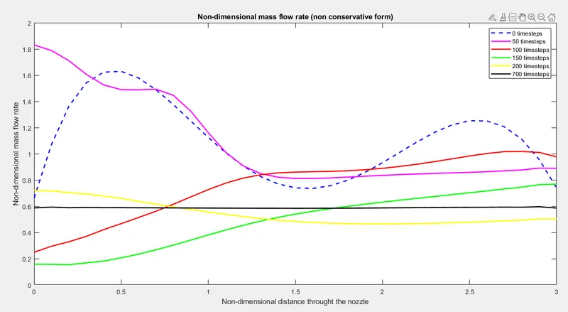
The non-dimensional mass flow is plotted as a function of non dimensional distance through the nozzle. Six different curves are shown, each for a different curve during the course of the time marching procedure. After 700 timesteps the mass flow distribution is a straight horizontal line across the graph. This says that the mass flow has converged to a steady state value throughout the nozzle.
Steady-state distribution of primitive variables inside the nozzle
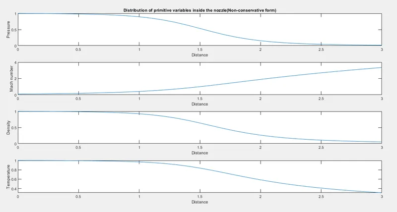
The graph shows the steady-state distribution of primitive variables inside the nozzle. We can see that the mach number is increasing as the flow proceeds through the nozzle. The pressure, density and temperature are decreasing with distance.
Time-wise variation of the primitive variables
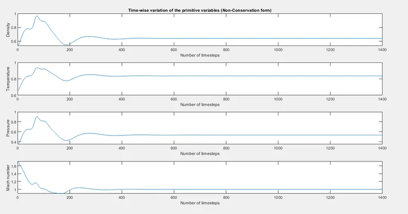
Time-wise variations of density, temperature, pressure and mach number at the nozzle throat. The largest changes take place at early times after which the final, steady state value is approached. At the beginning the flow field variables are driven by a stronger potential and hence changes rapidly. Later changes become much smaller with time as steady state is approached.
Conservation form
Variation of Mass flow rate distribution inside the nozzle at different time steps during the time-marching process
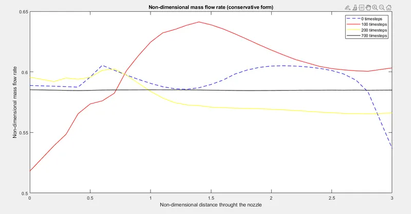
The dashed line represents the initial conditions. After 100 timesteps the mass flow deciates from the initial conditions. After 700 timesteps the mass flow is reaching almost a constant value, moreover it is quite close to the exact analytical value of 0.579.
Steady-state distribution of primitive variables inside the nozzle
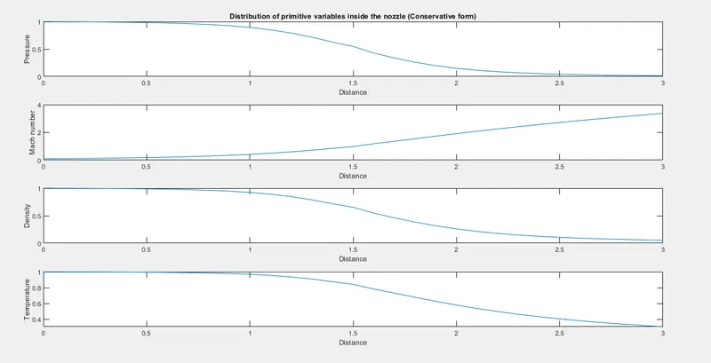
The graph shows the steady-state distribution of primitive variables inside the nozzle. We can see that the mach number is increasing as the flow proceeds through the nozzle. The pressure, density and temperature are decreasing with distance.
Time-wise variation of the primitive variables
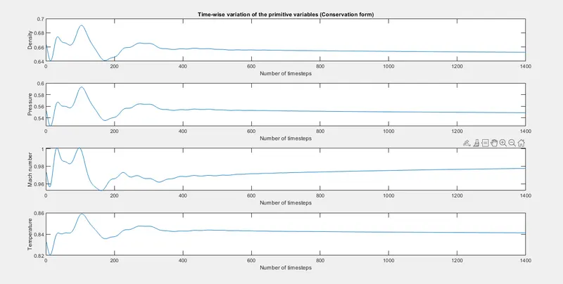
Large changes take place at the beginning, as the steady state is approached the changes are much smaller.
Comparison of Normalized mass flow rate distributions of both forms
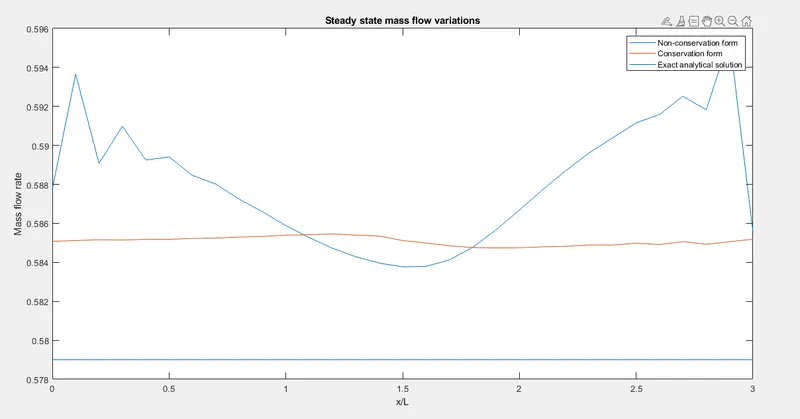
The graph shows the steady state mass flow variations obtained with the non-conservation and conservation forms of the governing equations. The steady state mass flow results obtained with the conservation form are much closer to the exact analytical solution of 0.579. The conservation form does a better job of preserving the mass throughout the flow field. The mass flow is a primary result in the conservation equations. The mass flow is only a secondary result in the non conservation equations.
Grid independency test
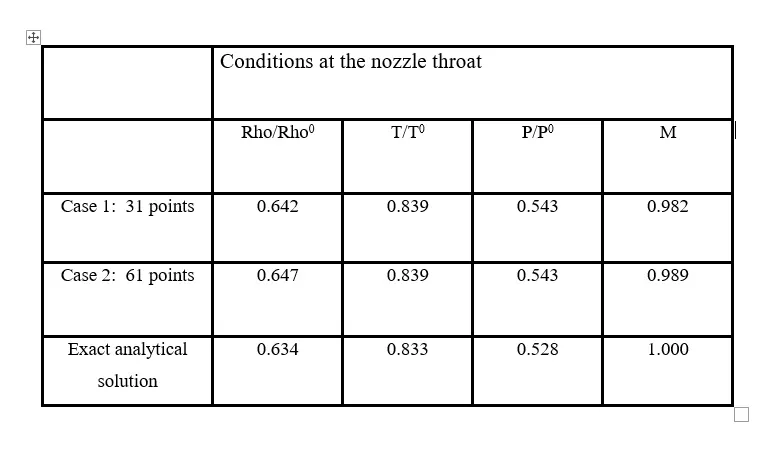
For different grid sizes even though the values are different at the beginning of the time marching procedure, it is almost same as stability is achieved. The results are very close to the analytical results.