Week 5 - Rayleigh Taylor Instability
AIM
To conduct the Rayleigh Taylor Instability CFD simulation
OBJECTIVES
- What are some practical CFD models that have been based on the mathematical analysis of Rayleigh Taylor waves? In your own words, explain how these mathematical models have been adapted for CFD calculations.
- Perform the Rayleigh Taylor instability simulation for 2 different mesh sizes with the base mesh being 0.5 mm. Compare the results by showing the animations( Attach them from your google drive). Observe the differences in the animation and explain the effect of mesh size on simulation. Also, explain why a steady-state approach might not be suitable for these types of simulation.[ Choose Air and Water for this simulation]
- Run one more simulation with water and user-defined material(density = 400 kg/m3, viscosity = 0.001 kg/m-s) for refined mesh.
- Define the Atwood Number. Find out the Atwood number for both the cases and explain how the variation in Atwood number in the above two cases affects the behavior of the instability.
THEORY
Rayleigh Taylor Instability (RTI)
In Multiphase flow, the dynamic variables like the velocity, viscosity, pressure and density are generally used to explain the movement of fluids under the gravitational field. Multiphase flows takes place in nuclear geothermal power plants, food processing industries and many others. One of the basic example is Rayleigh Taylor Instability. The Rayleigh Taylor Instability is a hydrodynamic instability arises when a high density fluid is placed over a low density fluid in a gravitational field. The RTI phenomenon was initially introduced by Rayleigh 1883 and later was observed for all accelerated fluids by Taylor 1950. When the density interface is disturbed, the hydrostatic pressure is generated, so the heavier fluid moves downwards and mixes with the lighter one, with the amplitude of perturbation initially growing exponentially but after sometime saturates and forms characteristic mushroom shape. When a heavier fluid is displaced downward with an equal volume of lighter fluid displaced upwards, it results in decrease of potential energy than it’s initial state. This RTI has been applied to a wide range of problems including the mushroom clouds like volcanic eruptions, nuclear explosions and plasma fusion reactors instability. The governing equations for The RTI problem are the Navier–Stokes equations, the continuity and the Cahn-Hilliard equations which are the non-dimensional form.
Examples include the behavior of water suspended above oil in the gravity of Earth, mushroom clouds like those from volcanic eruptions and atmospheric nuclear explosions, supernova explosions in which expanding core gas is accelerated into denser shell gas, instabilities in plasma fusion reactors and inertial confinement fusion.
Water suspended atop oil is an everyday example of Rayleigh–Taylor instability, and it may be modeled by two completely plane-parallel layers of immiscible fluid, the more dense on top of the less dense one and both subject to the Earth's gravity. The equilibrium here is unstable to any perturbations or disturbances of the interface: if a parcel of heavier fluid is displaced downward with an equal volume of lighter fluid displaced upwards, the potential energy of the configuration is lower than the initial state. Thus the disturbance will grow and lead to a further release of potential energy, as the more dense material moves down under the (effective) gravitational field, and the less dense material is further displaced upwards.
Some practical CFD models that have been based on the mathematical analysis of Rayleigh Taylor waves are;
Richtmyer–Meshkov instability
The Richtmyer–Meshkov instability (RMI) occurs when two fluids of different density are impulsively accelerated. Normally this is by the passage of a shock wave. The development of the instability begins with small amplitude perturbations which initially grow linearly with time. This is followed by a nonlinear regime with bubbles appearing in the case of a light fluid penetrating a heavy fluid, and with spikes appearing in the case of a heavy fluid penetrating a light fluid. A chaotic regime eventually is reached and the two fluids mix. This instability can be considered the impulsive-acceleration limit of the Rayleigh–Taylor instability.
Kelvin–Helmholtz instability
The Kelvin–Helmholtz instability (after Lord Kelvin and Hermann von Helmholtz) typically occurs when there is velocity shear in a single continuous fluid, or additionally where there is a velocity difference across the interface between two fluids. A common example is seen when wind blows across a water surface; the instability constant manifests as waves. Kelvin-Helmholtz instabilities are also visible in the atmospheres of planets and moons, such as in cloud formations on Earth or the Red Spot on Jupiter, and the atmospheres (coronas) of stars, including the sun's.
Plateau–Rayleigh instability
The Plateau–Rayleigh instability, often just called the Rayleigh instability, explains why and how a falling stream of fluid breaks up into smaller packets with the same volume but less surface area. It is related to the Rayleigh–Taylor instability and is part of a greater branch of fluid dynamics concerned with fluid thread breakup. This fluid instability is exploited in the design of a particular type of ink jet technology whereby a jet of liquid is perturbed into a steady stream of droplets. The driving force of the Plateau–Rayleigh instability is that liquids, by virtue of their surface tensions, tend to minimize their surface area. A considerable amount of work has been done recently on the final pinching profile by attacking it with self-similar solutions
Atwood number
The Atwood number (A) is a dimensionless number in fluid dynamics used in the study of hydrodynamic instabilities in density stratified flows. It is a dimensionless density ratio defined as
`A = (rho_1-rho_2)/(rho_1+rho_2)`
where
`rho_1` = density of heavier fluid
`rho_2` = density of lighter fluid
Simulation procedure
Preprocessing and Mesh
Open Ansys Workbench, select fluid flow(fluent) and create geometry in spaceclaim.
At first, geometry is created as square boxes and converted to surface using Pull tool and share topology is turned on.
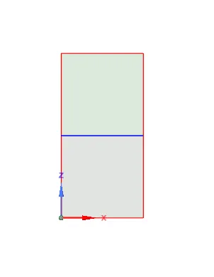
After creating geometry, close spacelaim then the next step is to create the mesh.
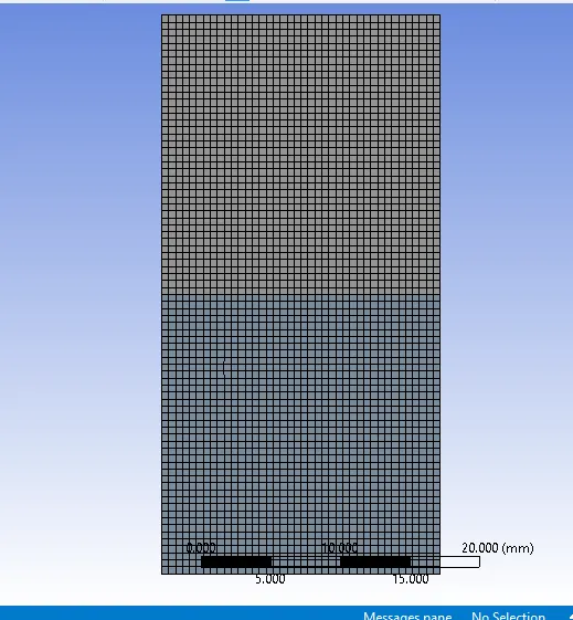
Meshing is complete. Double click on setup to open CFD solver.
CFD Case Setup
• Pressure based solver and Absolute velocity is used.
• Transient-state Calculation is performed.
• Compressible fluid flow is chosen.
• Gravity is enabled in -ve Y axis.
• Multiphase Model is turned on along with Volume of Fluid and number of Eulerian phases is chosen as 2 and Implicit scheme is selected.
• Viscous model-Laminar is used.
• Cell zone selected as Fluid-air;water-surface:water-liquid
• Patching of the volume fraction of the two phases is performed before the start of simulation. Phase used for patching was water and volume fraction of 1 is taken for water surface and 0 for air surface.
Results
Case 1
Water and Air (`rho_(water) = 998.2 (kg)/m^3`, `rho_(air) = 1.225 (kg)/m^3`)
Baseline mesh
Mesh size = 0.5mm
Number of elements = 3200
Residual plot
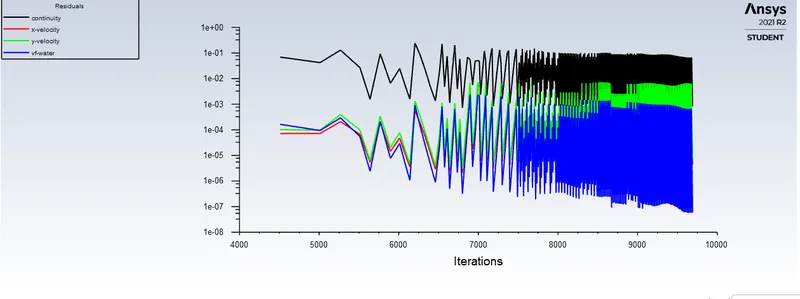
The animation video is given in the below link;
https://drive.google.com/file/d/1B8sUr3A5zyltcWMU5Xa2QwzubuTGtOuC/view?usp=sharing
Case 2
Water and Air
Refined mesh
Mesh size = 0.1mm
Number of elements = 80000
Residual plot
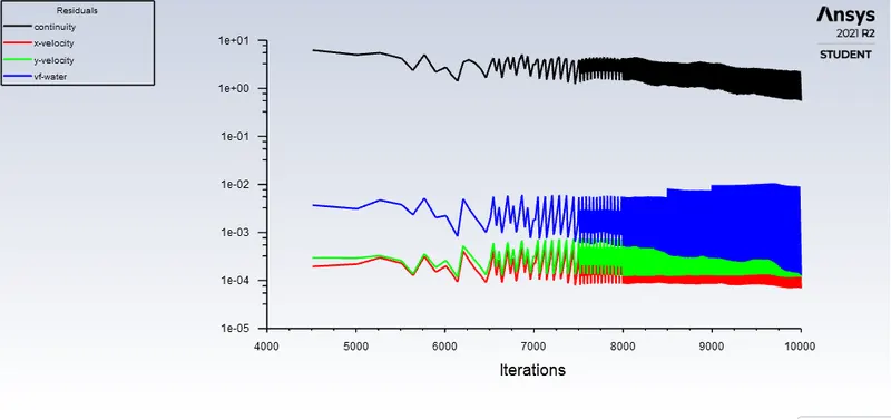
The animation video is given in the below link;
https://drive.google.com/file/d/1hbO8IqI_wr4i30tAnmosSMo3C_DALG-8/view?usp=sharing
Case 3
Water and User defined material (density = 400 kg/m3, viscosity = 0.001 kg/m-s)
Refined mesh
Mesh size = 0.1mm
Number of elements = 80000
Residual plot
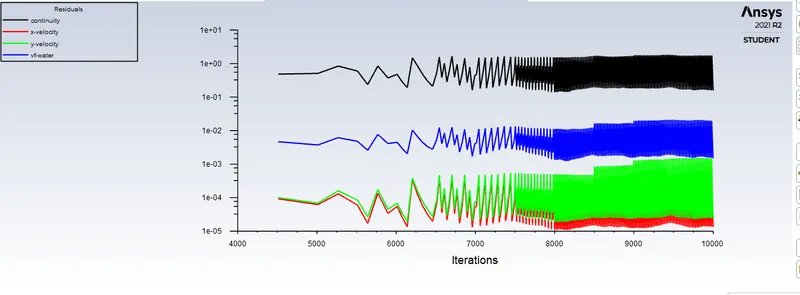
The animation video is given in the below link;
https://drive.google.com/file/d/1VUaECip-0X-I_XRANWPylODRRLYrUDs-/view?usp=sharing
- Explain why a steady-state approach might not be suitable for these types of simulation?
For Transient simulation, compared to steady state, has higher demand in terms of
computational time. Transient solver better captures the flow and can be used to run at smaller time steps. Smaller time steps are required to observe the instabilities and can be only possible through transient simulation. Since it is a time marching solution, we expect more accuracy from
transient simulation for which Transient simuation is the ideal setup to run the calculation for Rayleigh Taylor Instability. Steady state approach cannot be used where changes are happening with respect to time.
Atwood number for water and air mixture = 0.9975
Atwood number for water and user defined material = 0.4278
For Atwood number closer to 1, means the lighter fluid below the heavier fluid takes the form of larger bubble like plumes. The light fluid moves into the heavy fluid in the form of round topped bubbles with circular cross section. For A closer to 0, RTI flows take the form of symmetric 'fingers' of fluid. Thus the variation in Atwood number in the above two cases affects the behavior of the instability.
CONCLUSION
- Rayleigh taylor instability is a fingering instability of an interface between two fluids of different densities. Basically it is a battle between two fluids of different densities when the lighter fluid pushes the heavier fluid.
- A simulation on RTI was conducted with different cases, the first case involving air, water and the second case with water and a user defined material. The simulation was conducted with baseline mesh and refined mesh.
- When the mesh is refined, the results are more smooth. We get a better view of the irregularities that takes place at the interface with refined mesh. The refined mesh captures the instability better. The computational time required is more but the accuracy is higher for the refined mesh.
- For time marching problem, transient approach is more suitable than the steady state approach.
- The Atwood number helps in finding the behaviour of the instability.
- Numerous factors influence the development of Taylor instability in a simple fluid. These include surface tension, viscosity, compressibility, effect of converging geometry, three-dimensional effects, time dependence of the driving accelerations, shocks.