Week 10: Project 1 - FULL HYDRO case set up (PFI)

AIM

PFI engine simulation using converge

Engine Geometric Parameters

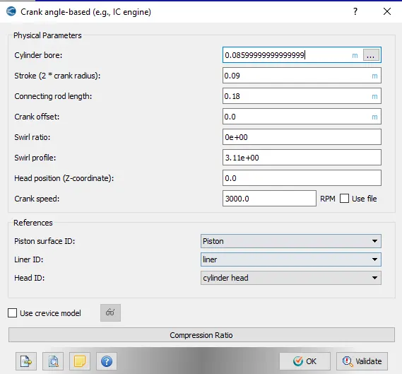
1. Bore =0.086 m
2. Stroke = 0.09 m
3. Connecting rod length = 0.18 m
4. RPM = 3000

Run parameters

1. Simulation mode: No Hydro

Simulation time parameters

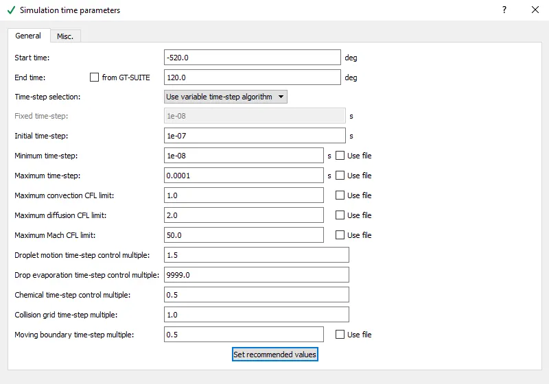
1. Start time : -520 deg
2. end time : 120 deg

Boundary conditions

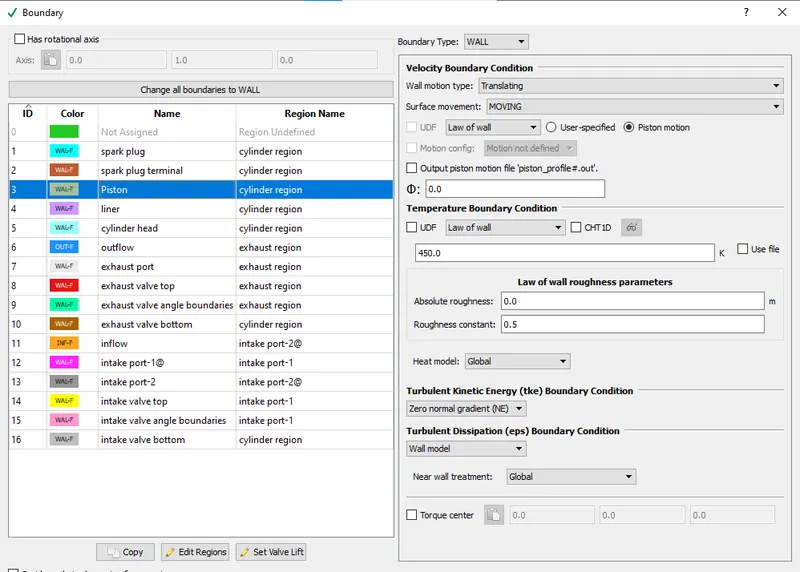
1. Piston temperature - 450K
2. Liner temperature - 450K
3. Head temperature - 450K
4. Spark Plug temperature - 550K
5. Spark Plug electrode temperature - 600K
6. Exhaust ports temperature - 500K
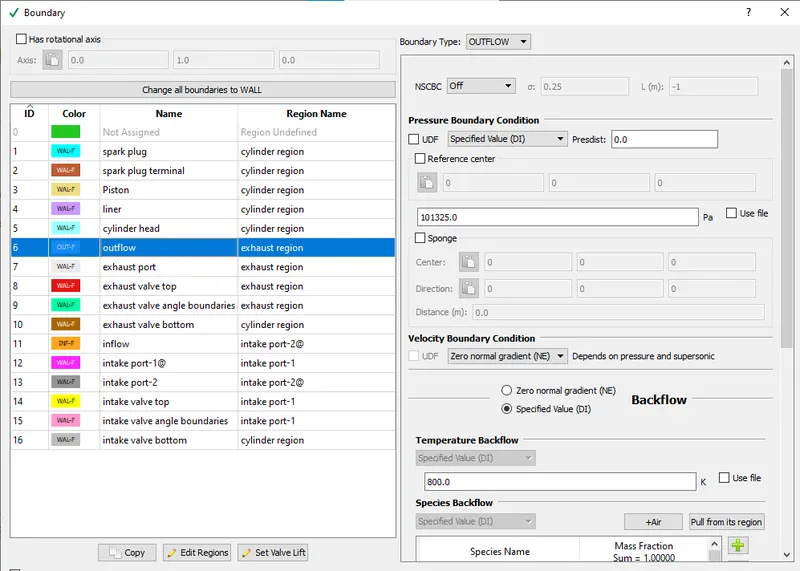
7. Exhaut outflow - 1 bar
8. Exhaust outlflow temperature - 800k
9. Exhaust species concentration - Calculate the stoichiometric condition
10. Exhaust valve top temperature - 525K
11. Exhaust valve angle temperature - 525K
12. Exhaust valve bottom temeprature - 525K
13. Intake port - 1 temperature 425K
14. Intake port - 2 temperature 425K
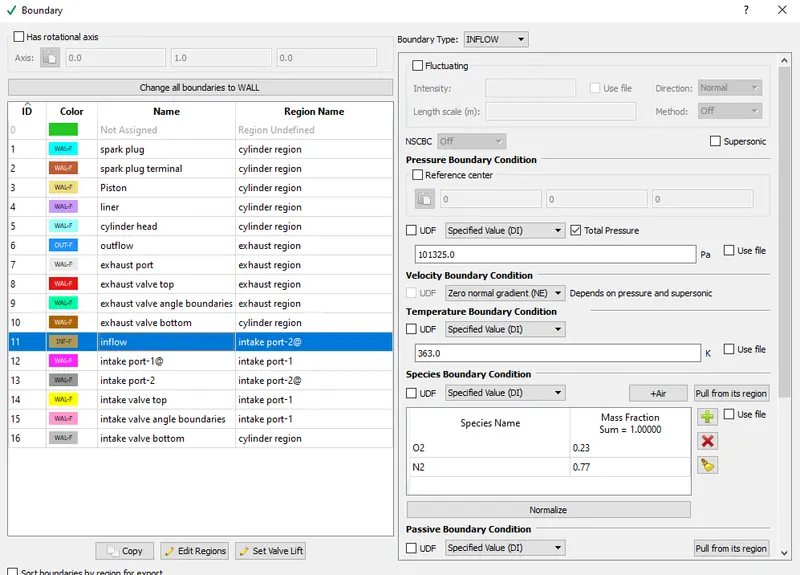
15. Inflow pressure - 1 bar total pressure
16. Inflow temperature - 363K
17. Inflow species - Air
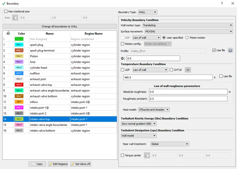
18. Intake valve top temperature - 480K
19. Intake valve angle temperature - 480K
20. Intake valve bottom temeprature - 480K

Initial conditions

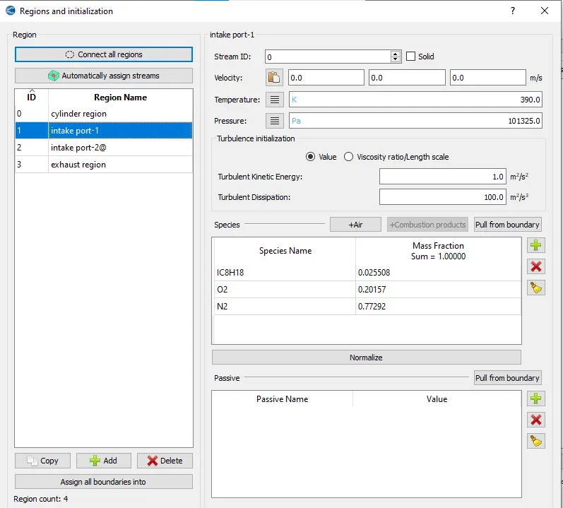
• Intake port - 1 (closer to combustion chamber)
  • ic8h18 - 0.025508
  • o2 - 0.20157
  • n2 - 0.77292
  • Temperature - 390k
  • pressure - 1 bar
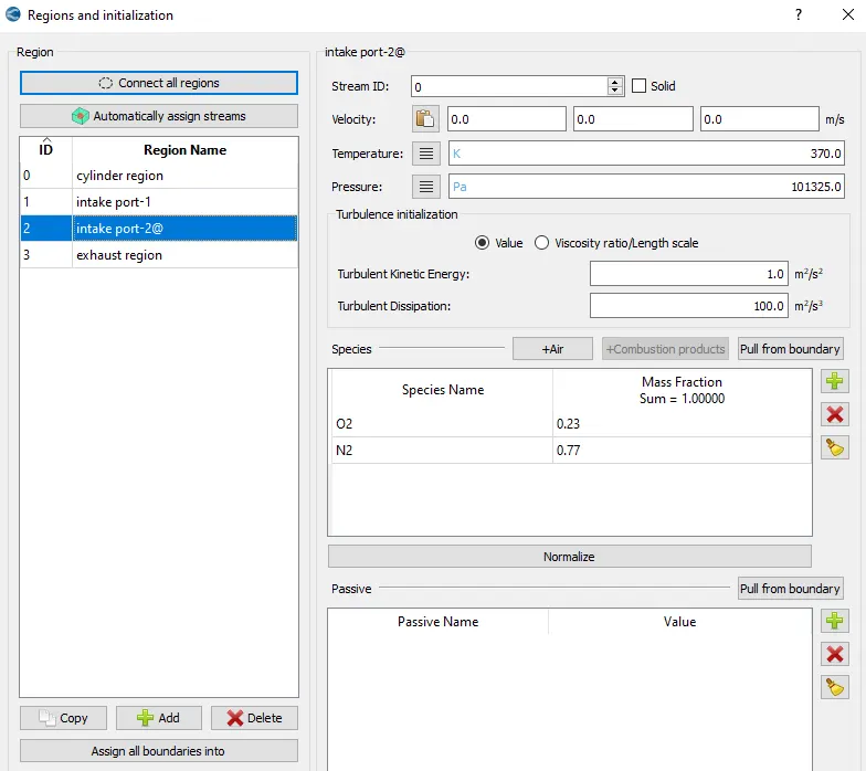
• Intake port - 2 (away from combustion chamber)
  • Air
  • Temperature - 370K
  • Pressure - 1 bar
• Cylinder
  • Pressure - 1.85731 bar
  • Temperature - 1360K
  • Stoichiometric composition

Injection Parameters

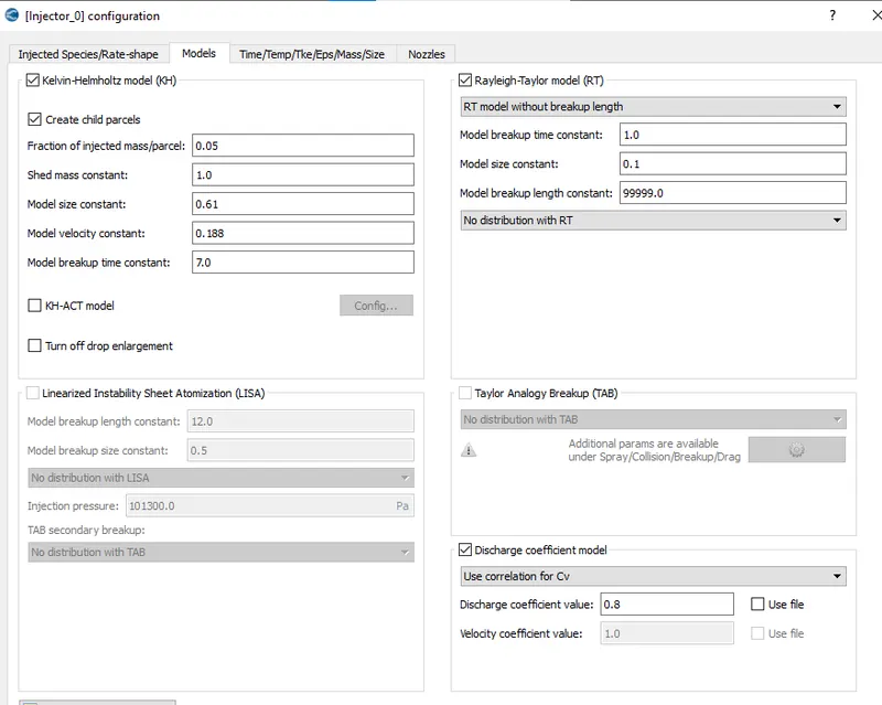
1. Fuel flow rate = 7.5e-4 Kg/second
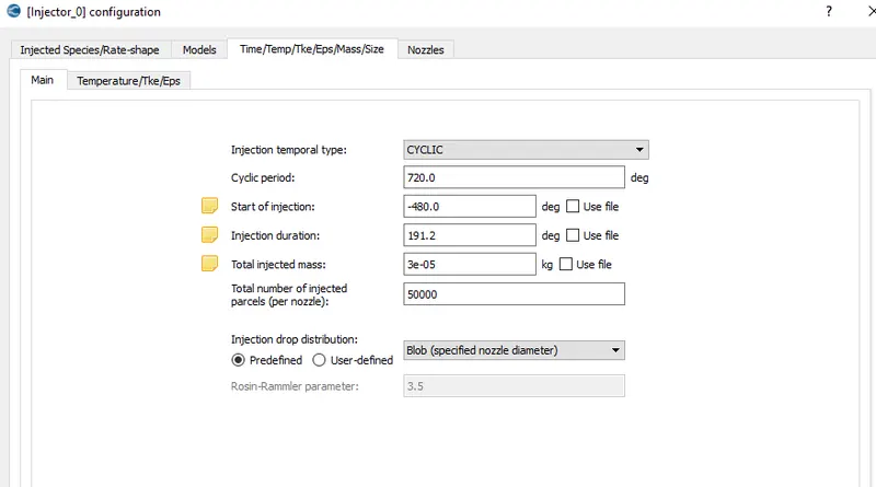
2. Injection start time = -480.0
3. Injection duration = 191.2
4. Fuel temperature = 330K

Nozzle positions

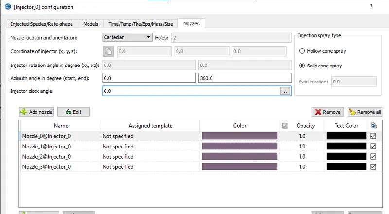
Nozzle diameter = 250 micro-meter

Circular injection radius = Nozzle radius

Spray cone angle = 10

• Nozzle 0
  • center 0.0823357 0.00100001 0.07019
  • Align Vector -0.732501 0.210489 -0.647408
• Nozzle 1
  • center 0.0823357 -0.00099999 0.07019
  • Align Vector -0.732501 -0.210489 -0.647408
• Nozzle 2
  • center 0.0823357 -0.0004 0.07019
  • Align Vector -0.5 -0.2 -0.647408
• Nozzle 3
  • center 0.0823357 0.0003 0.07019
  • Align Vector -0.5 0.2 -0.647408

Spark Ignition Parameters

• Start of spark = -15 deg
• Spark duration = 10 deg
• Spark location = -0.003 0 0.0091
• Spark radius = 0.0005m

OBJECTIVE

To run a PFI engine simulation with above given parameters

SIMULATION PROCEDURE

1. Setting up the case in converge
2. Running the simulation in cygwin
3. Post convert using cygwin/converge
4. Post processing in paraview

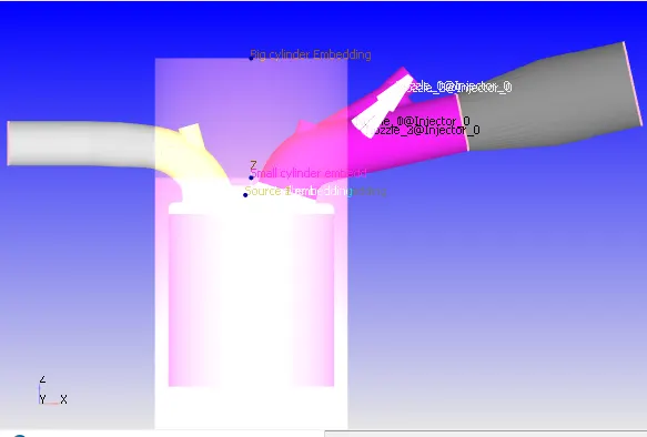
The physical parameters are entered as given below:

Simulation time parameters

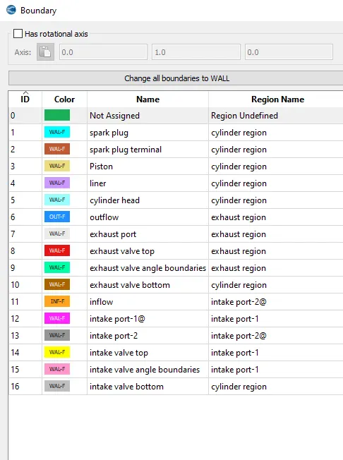
Boundary conditions

Piston

Inflow

Outflow

Intake valve top, angle and bottom

These three surfaces have exact same boundary conditions and valve motion is defined using a file 'intake_lift.in'.

Exhaust valve top,angle and bottom

These three surfaces have exact same boundary conditions and valve motion is defined using a file 'exhaust_lift.in'.

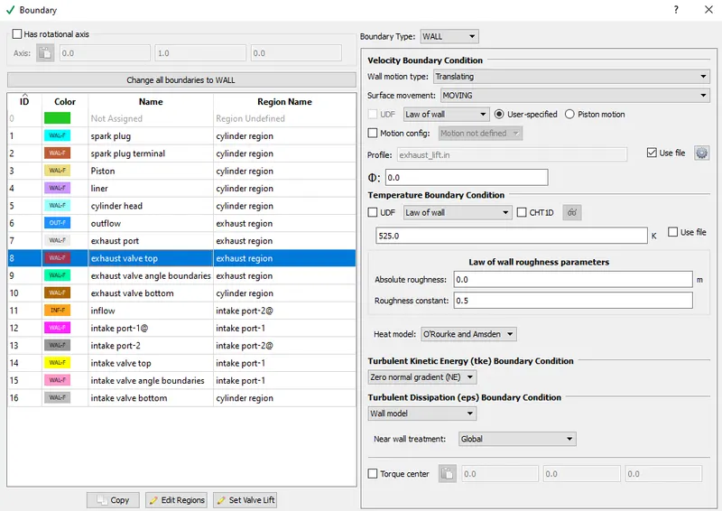
All other boundaries are fixed wall boundaries. Only difference is in the temperature boundary condition.

cylinder head - 450K

liner - 450K

Spark plug - 550K

Spark plug electrode - 600K

Exhaust port - 500K

Intake port-1 and intake port-2 - 425K

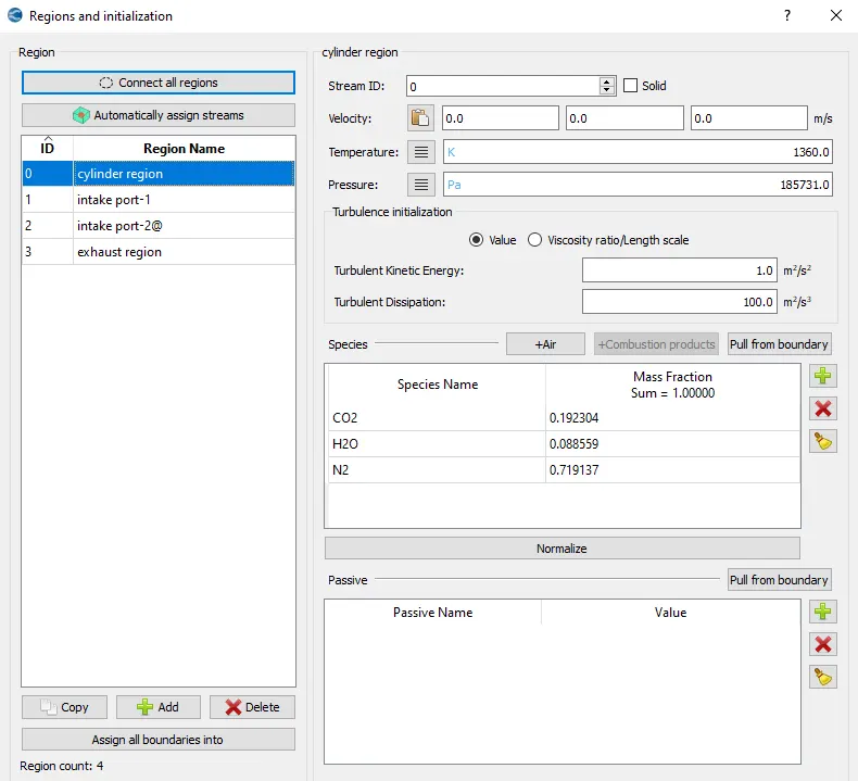
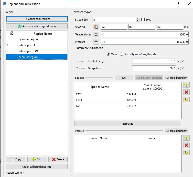
Regions and Initialisation

The fuel used is isooctane (IC8H18)

The equation for combustion of this fuel,

`C_8H_18 + 12.5(O_2+3.76N_2)= 8CO_2 + 9H_2O + (3.76*12.5)N_2`

From this equation the mass fraction of each species is found out.

`CO_2`= 0.192304

`H_2O` = 0.088559

`N_2` = 0.719137

Cylinder region

Intake port-1

Intake port-2

Exhaust region

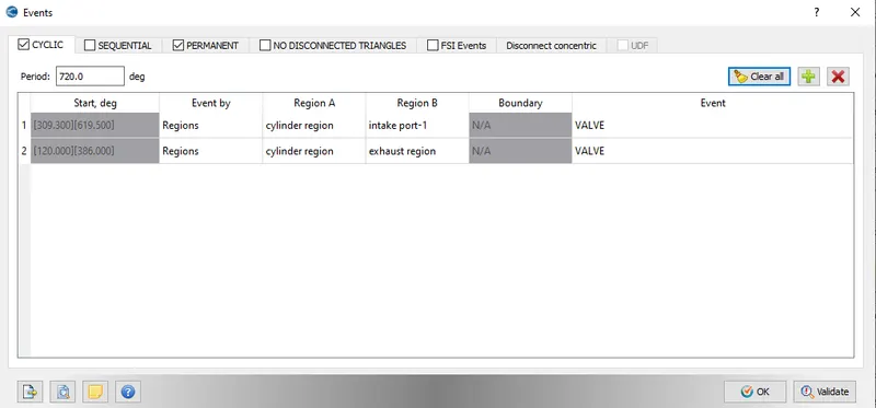
Events

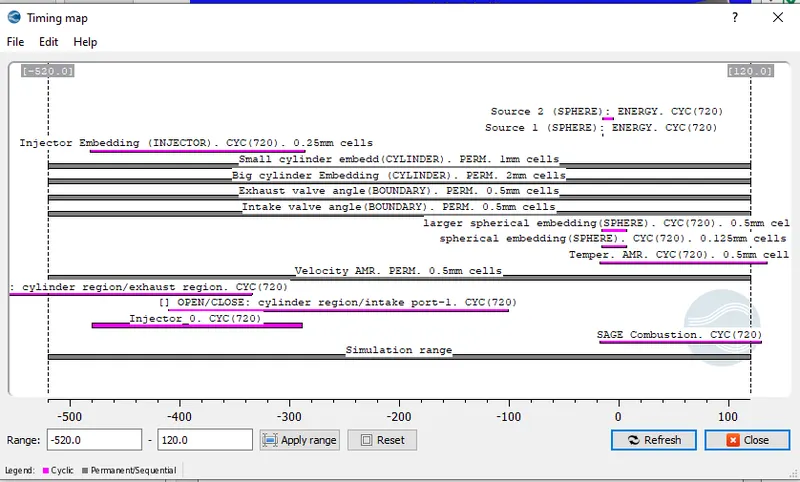
Using cylic option in the events tab, intake port-1 and exhaust region are connected and disconnected with the combustion chamber based on valve timing.

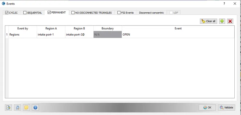
These two regions are always open to each other.

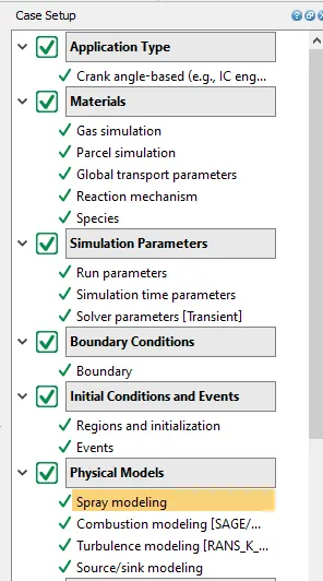
In this simulation the important steps are spray modelling, combustion modelling and source/sink modelling.

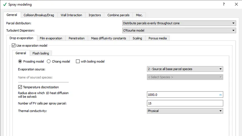
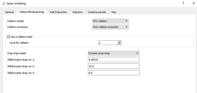
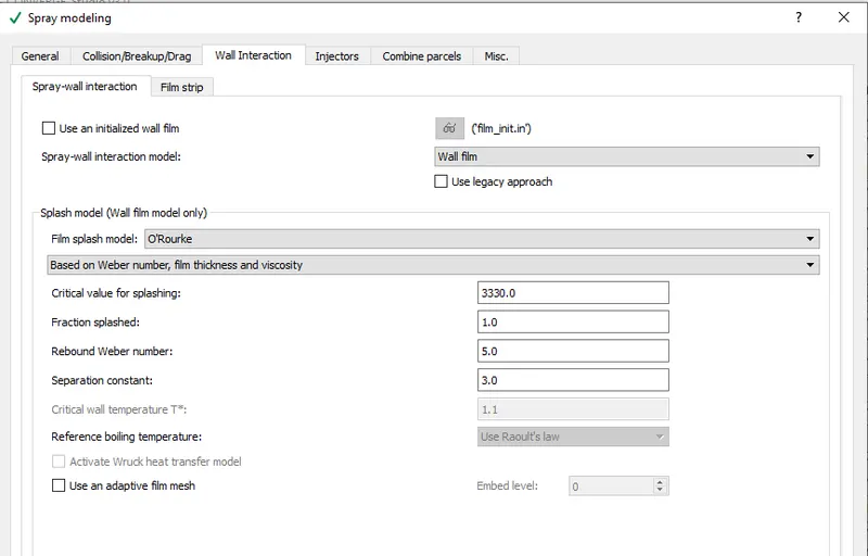
Spray modelling

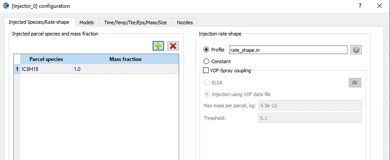
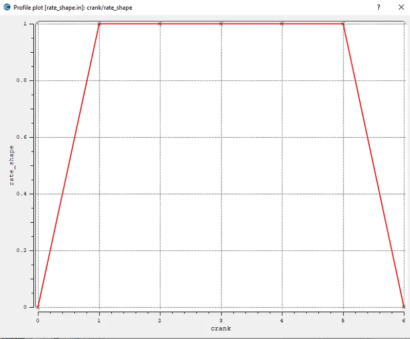
Iso-octane is used as the fuel. Add iso-octane in the parcel simulation. The parcels are set to distribute evenly throughout the cone. O'Rourke model is chosen for turbulent dispersion.

Combustion modelling

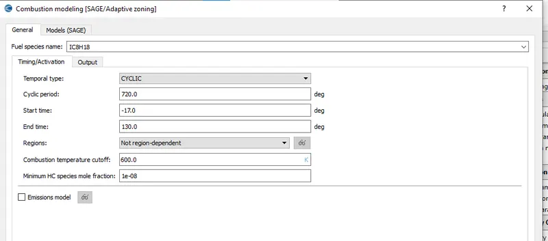
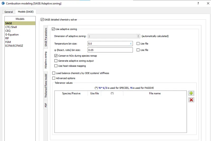
The combustion is started few crank angles before the spark. So that the combustion solver is ready to solve it. The end time is determined by the degree to which the exhaust valve opens. Adaptive zoning is used to solve the combustion faster.

Source/sink modelling

In a spark ignition engine, the fuel is mixed with air and then inducted into the cylinder during the intake process. After the piston compresses the fuel-air mixture, the spark ignites it, causing combustion. The expansion of the combustion gases pushes the piston during the power stroke. So for simulating the combustion the source of power should be specified.

• Spark location = -0.003 0 0.0091
• Spark radius = 0.0005m

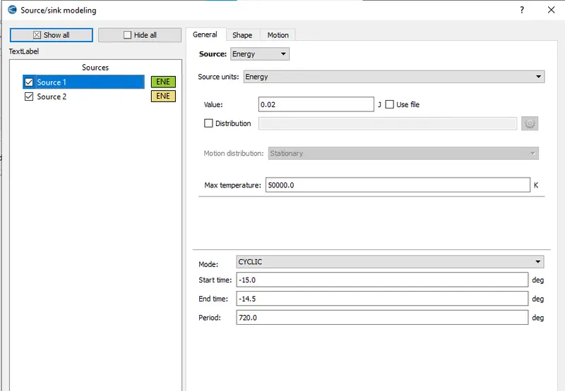
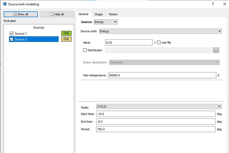
The spark ignition can be divided into three phases. The breakdown, arc and glow phase. In the first phase more energy is put in. That is 40MJ of energy is introduced to initiate the spark and then 20 MJ is maintained. In the source modelling, 2 sources are added. The first energy source takes place for 0.5deg of crank angle time and the next source takes place for 10deg.

Turbulence modelling

Timing map

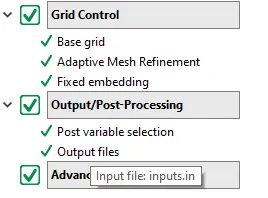
Case setup tree

RESULTS

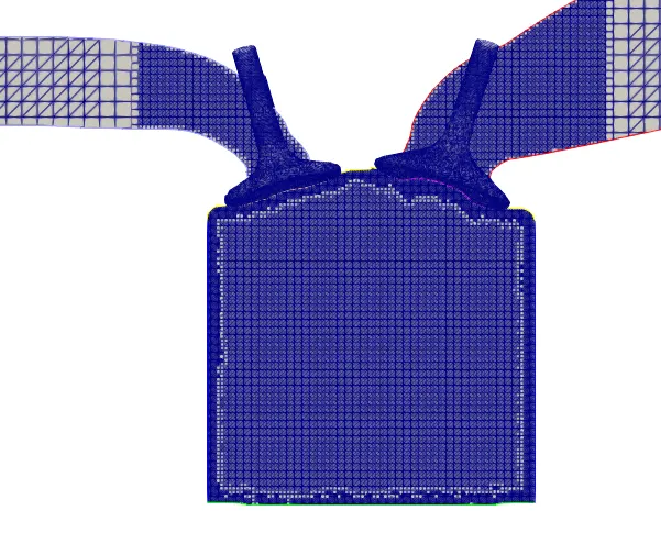
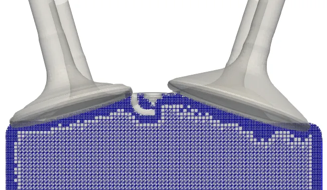
Mesh

https://youtu.be/hYsFo9oOC0k

Volume plot

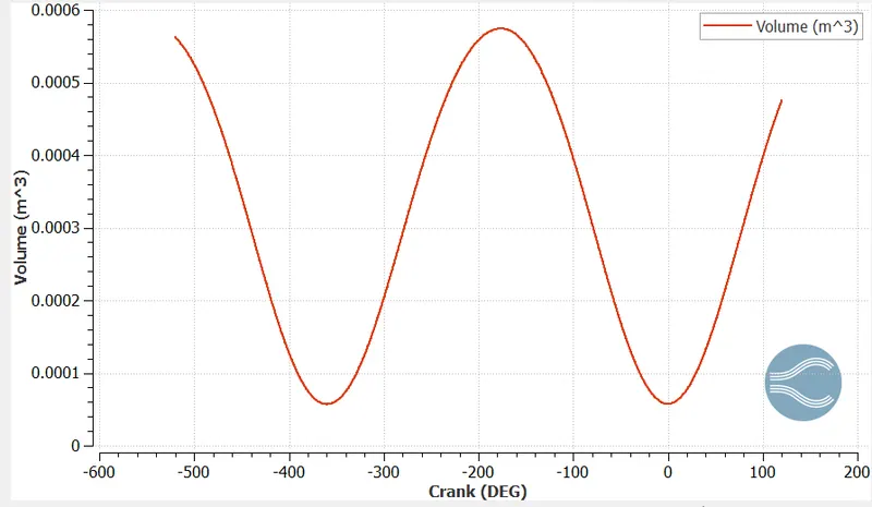
The volume of the combustion chamber increases and decreases at the same rate during the upstroke and downstroke. The movement of the piston controls the volume of the combustion chamber. From this plot the compression ration of the engine can be calculated.

Compression ratio = maximum volume/minimum volume

= `0.00096185157/(0.00096185157)`

= 2.185

Pressure plot

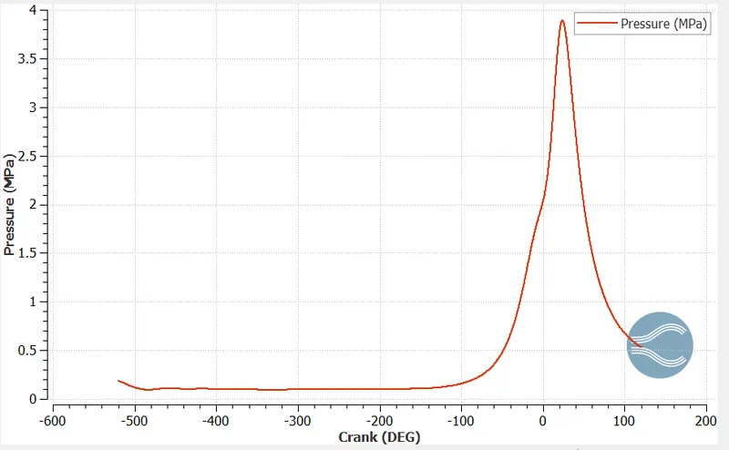
The pressure varies only a little at the beginning. Then there is a sudden rise and fall of the pressure. The pressure varies a little until the ignition occurs. After ignition the pressure inside the combustion chamber increases at a faster rate and reaches a maximum value. The ignition occurs at the end of the compression stroke.

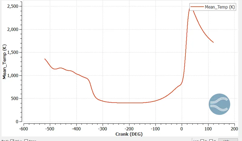
Temperature plot

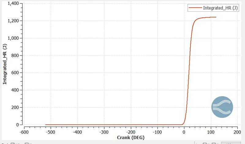
Integrated heat release

Amount of emission

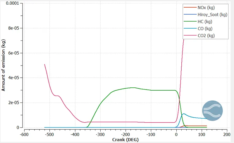
This plot shows the amount of emission occuring in an IC engine. There is a high level of CO2 emission at the exhaust. The emissions produced can be reduced by improving the combustion.

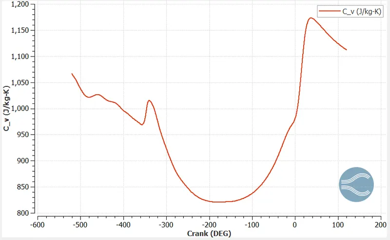
Change in specific heat in constant volume

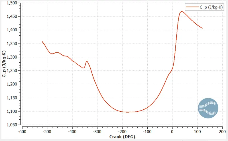
Change in specific heat in constant pressure

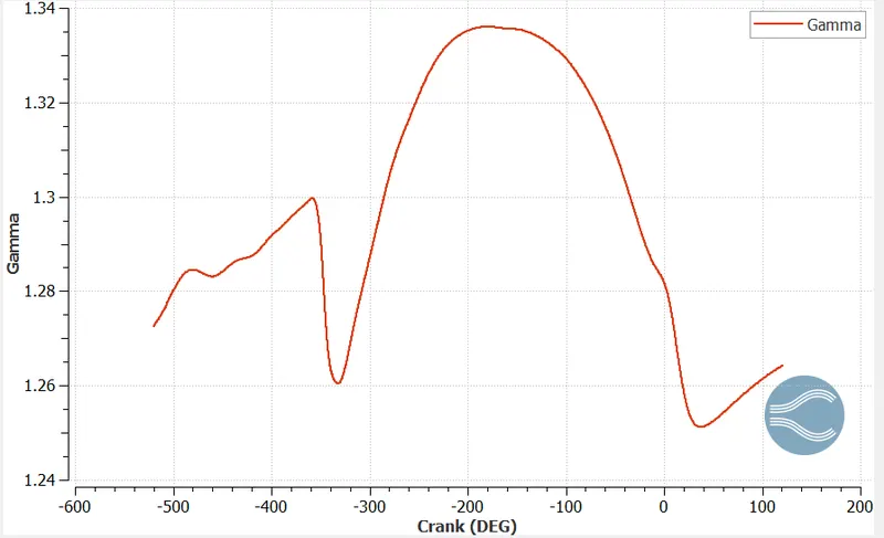
Gamma plot

Combustion efficiency

`eta_c = (IHR)/(m_f*CV)`

where `m_f`, amount of fuel added = `3*10^-5`kg per cycle

CV, calorific value of fuel = 44*10^6 J/kg

`eta_c` = `1241.1646/((3*10^-5)*44*10^6)`

= 0.94

= 94%

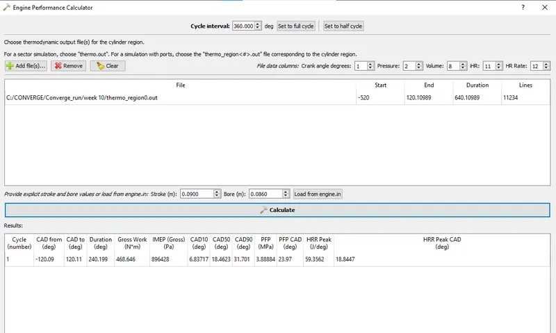
Power calculation

Work = 486.646Nm

RPM = 3000

RPS = 3000/60 = 50

Total degree per sec = 50 * 360 = 18000

Time in sec = 240.199/18000

= 0.01334 sec

Power = W/t

= 486.646/0.01334

= 35130.88KJ

= 35.13KW

Torque

P = `(2*pi*N*T)/60`

T = `(P*60)/(2*pi*N)`

= `(35.13*10^3*60)/(2*pi*3000)`

= 111.879Nm

• Why do we need a wall heat transfer model? Why can't we predict the wall temperature from the CFD simulation?

Internal combustion engines are now extremely optimized, in such ways improving their performance is a costly task. Traditional engine improvement by experimental means is aided by engine thermodynamic models, reducing experimental and total project costs. For those models, accuracy is mandatory in order to offer good prediction of engine performance. Modelling of the heat transfer and wall temperature is an important task concerning the accuracy and the predictions of any engine thermodynamic model, although it is many times an overcome task. In order to perform good prediction of engine heat transfer and wall temperature, models are required for accomplish heat transfer from hot gases to engine parts, heat transfer inside each engine part, and also heat transfer to coolant and lubricating oil.

• What is the significance of ca10, ca50 and ca90?

ca10, ca50 and ca90 are the crank angles at which the cumulative heat release reaches at 10%, 50% and 90%.The physical significance of ca10 is that it is used to identify the start of ignition in an engine, ca50 indicates the end of premixed combustion and the start of diffused combustion. ca10-ca90 gives the combustion duration.

Temperature animation :

https://drive.google.com/file/d/1wIwwM0EYScneO-HwsMR9-D2HHcB9-OUg/view?usp=sharing

Pressure animation :

https://drive.google.com/file/d/1GNkCohy5cy8XDUUaWulCBjVgDoBWUbdF/view?usp=sharing

IC8H18 fuel spray animation :

https://drive.google.com/file/d/1PAk5OVOGYBhvLkBIfzdPP0-3KjIvWKrr/view?usp=sharing

CONCLUSION

Succesfully simulated the PFI full hydro case of the engine. Using engine performance calculator the power and torque of the engine was calculated.