Week 3 - Solving second order ODEs
Link of animated video is given below-
First of all we have the 2nd order ODE for a simple pendulum motion. Now we will make this 2nd order ODE in two different 1st order ODE.
. So the 2nd order ODE is `(d^2theta)/dt^2+b/m(d theta)/dt+g/lsintheta=0`.
let asume `theta=theta1`. So we can say `(d theta)/dt=(d theta1)/dt`. And also asume that `(d theta1)/dt=theta2......(i)`.
From equation (i) we can write `(d^2theta)/dt^2=(d^2theta)/dt^2=d/dt((d theta1)/dt)=d/dt(theta2)=(d theta2)/dt`.
so, `(d^2theta)/dt^2=(d theta2)/dt.......(ii)`.
So by putting equation (i) and (ii) into 2nd order ODE we will get `(d theta2)/dt+b/mtheta2+g/lsintheta1=0`.
or, `(d theta2)/dt=-b/mtheta2-g/lsintheta1.......(iii)`.
So hera equation (i) represents the velocity of the pendulum and equation (iii) represents the acceleration. So we have to find out the solution for equation (i) and (iii). If we arange that solution it looks like below
`d/dt[[theta1],[theta2]]=[[theta2],[-b/mtheta2-g/lsintheta1]]`.
Now we will go the coading part for 2nd order ODE solution. so we have some given data, that are length of string(`l`) is 1 meter, mass(`m`) of ball is 1kg, Damping coefficient(`b`) is 0.05 and gravity(`g`) is `9.81m//s^2`. And initial angular velocity is `3rad.//sec.` and initial displacement is 0 at the time `t=0`(means when pendulum not started moving). we have to simulate the motion of time between 0sec to 20sec.
So at first we will make function to solve our ODE by using 'function' command. Here our function name will be 'ode_func'. Number of output of this function will be 2 in column and 1 in row. Inputs are 6 and they are t(time), theta(anguler displacement), b, g, l, m. so the function will look like
function dtheta_dt=ode_func(t,theta,b,g,l,m)
theta1=theta(1)
theta2=theta(2)
dtheta1_dt=theta2
dtheta2_dt=-(b/m)*theta2-(g/l)*sin(theta1)
dtheta_dt=[dtheta1_dt;dtheta2_dt]
end
after successfully saving the function we will go for main coadding part. starting with defining all given inputs, make sure initial value of displacement and velocity are written in correct way and simulation time span is correct. after that we will use 'ode45' function to solve this ODE. It is a MATLAB inbuilt function that is used for solving ODE of 2nd order, 3rd order and higher orders also. Here we will get two output, one is time(t) that is a 500x1 matrix(500 row means in between time span we have taken 500 values) and another is a 500x2 matrix result where 1st row define the all angular displacement values and second row define the angular velocity of the pendulum. So the code will be
clear all
close all
clc

%inputs
b=0.05
m=1%kg
g=9.81%m/s^2
l=1%meter

%initial condition
theta_0=[0;3]

%time points
t_span=linspace(0,20,500)


% solve ODE

[t, results]=ode45(@(t,theta) ode_func(t,theta,b,g,l,m),t_span,theta_0)
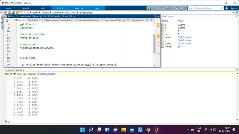
So from the results we can see how angular displacement and angular velocity changes with tespect of time. If we plot the graph of time vs displacement and time vs velocity it will like
clear all
close all
clc

%inputs
b=0.05
m=1%kg
g=9.81%m/s^2
l=1%meter

%initial condition
theta_0=[0;3]

%time points
t_span=linspace(0,20,500)


% solve ODE

[t, results]=ode45(@(t,theta) ode_func(t,theta,b,g,l,m),t_span,theta_0)


plot(t,results(:,1))
hold on
plot(t,results(:,2))
xlabel('time')
ylabel('displacement & velocity')
legend('angular displacement','velocity')
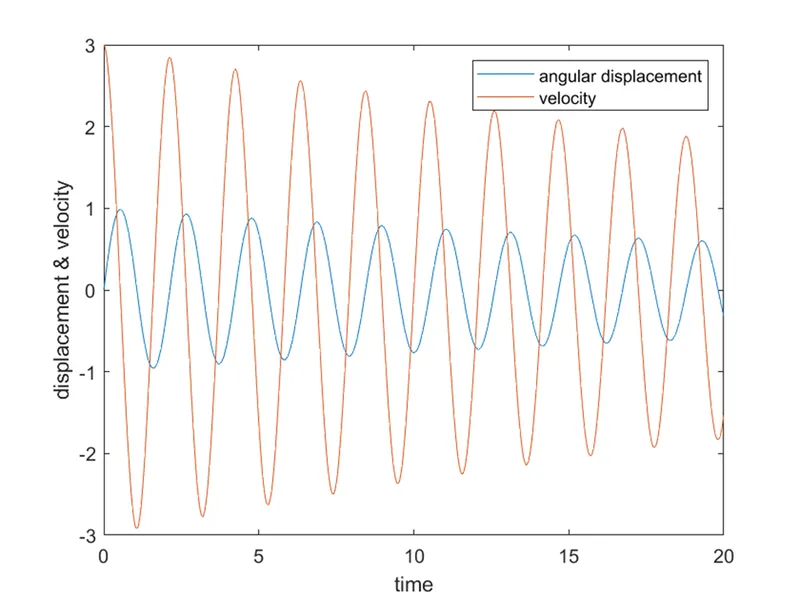
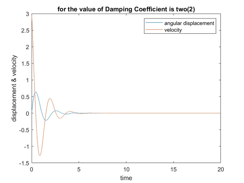
So from the graph we can see velocity starting from 3rad/sec and decreasing with respect of time. Displacement starting from 0 and decreasing with respect of time but not so fast as velocity. This values can change if damping coefficient changes. suppose if we take damping coefficient 2 then velocity and displacement will decrease more fast. as an is given below
clear all
close all
clc

%inputs
b=2
m=1%kg
g=9.81%m/s^2
l=1%meter

%initial condition
theta_0=[0;3]

%time points
t_span=linspace(0,20,500)


% solve ODE

[t, results]=ode45(@(t,theta) ode_func(t,theta,b,g,l,m),t_span,theta_0)


plot(t,results(:,1))
hold on
plot(t,results(:,2))
xlabel('time')
ylabel('displacement & velocity')
legend('angular displacement','velocity')
title('for the value of Damping Coefficient is two(2)')
Now for simulating the pendulum we have to take two point, one is fixed(x0,y0) and the coordinate willbe (0,0). And another point(x1,y1) attached with a 1kg ball will change its place according to time.
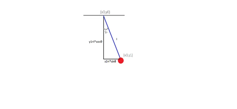
As we can see in this above picture we can calculate the value of x1 and y1 with different theta angle. Here theta angle is nothing but angular displacement that is given in 1st row and all 500 column of 'result' matrix. so we have to run a 'for' loop to execute all values of theta. And then have to use 'plot' command for ploting the pendulum and use 'pause' command for animation.
clear all
close all
clc

%inputs
b=0.05
m=1%kg
g=9.81%m/s^2
l=1%meter

%initial condition
theta_0=[0;3]

%time points
t_span=linspace(0,20,500)


% solve ODE

[t, results]=ode45(@(t,theta) ode_func(t,theta,b,g,l,m),t_span,theta_0)

theta=results(:,1)

for i=1:length(theta);
    x0=0
    y0=0
    x1=l*sin(theta(i))
    y1=l*cos(theta(i))

hold on
 fill([-l-0.2*l l+0.2*l l+0.2*l -l-0.2*l],[-l-0.2*l -l-0.2*l l+0.2*l l+0.2*l],'w');
plot([x0 x1],[y0 y1],'b','LineWidth',3);
   plot(x1,y1,'Marker','o','MarkerSize',20,'MarkerFaceColor','r','MarkerEdgeColor','r');
   plot([-0.5 0.5],[0 0],'LineWidth',5,'Color','black')
pause(0.0001)
end
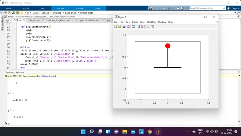
As we can see pendulum is not in its wright positon, because we have taken the fixed point of pendulum is (0,0) and y1 value is positive. So pendulum is simulating in y(positive) section. to correct this we have to take y1 value negative.
clear all
close all
clc

%inputs
b=1.5
m=1%kg
g=9.81%m/s^2
l=1%meter

%initial condition
theta_0=[0;3]

%time points
t_span=linspace(0,20,500)


% solve ODE

[t, results]=ode45(@(t,theta) ode_func(t,theta,b,g,l,m),t_span,theta_0)

theta=results(:,1)

for i=1:length(theta);
    x0=0
    y0=0
    x1=l*sin(theta(i))
    y1=-l*cos(theta(i))

hold on
 fill([-l-0.2*l l+0.2*l l+0.2*l -l-0.2*l],[-l-0.2*l -l-0.2*l l+0.2*l l+0.2*l],'w');
plot([x0 x1],[y0 y1],'b','LineWidth',3);
   plot(x1,y1,'Marker','o','MarkerSize',20,'MarkerFaceColor','r','MarkerEdgeColor','r');
   plot([-0.5 0.5],[0 0],'LineWidth',5,'Color','black')
pause(0.0001)
end
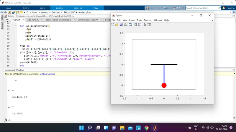
Now the pendulum is simulating in right position. By modifying the code we can make it more representable. And by using 'movie' command we can make a proper animation video of it. So the final code will be
clear all
close all
clc

%inputs
b=0.05
m=1%kg
g=9.81%m/s^2
l=1%meter

%initial condition
theta_0=[0;3]
%time points
t_span=linspace(0,20,500)


% solve ODE

[t, results]=ode45(@(t,theta) ode_func(t,theta,b,g,l,m),t_span,theta_0)

theta=results(:,1)

ct=1
for i=1:length(theta);
    x0=0
    y0=0
    x1=l*sin(theta(i))
    y1=-l*cos(theta(i))

figure(1)
hold on
 fill([-l-0.2*l l+0.2*l l+0.2*l -l-0.2*l],[-l-0.2*l -l-0.2*l l+0.2*l l+0.2*l],'w');
plot([x0 x1],[y0 y1],'b','LineWidth',3);
   plot(x1,y1,'Marker','o','MarkerSize',20,'MarkerFaceColor','r','MarkerEdgeColor','r');
   plot([-0.5 0.5],[0 0],'LineWidth',5,'Color','black')
pause(0.0001)

%figure(2)
%plot(t,results(:,1),"Color",'y')
%hold on
%plot(t,results(:,2),'g')
M(ct)=getframe(gcf)
ct=ct+1

end
movie(M)
videofile=VideoWriter('simple_pendulum_motion_animation.AVI','Uncompressed AVI');
open(videofile)
writeVideo(videofile,M)
close(videofile)