Week 4.1 - Genetic Algorithm
Optimising stalagmite function using GA (Gematric Algorithm)
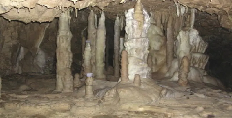
stalagmites: stalagmites are the most common speleothems(Speleothems are secondary mineral deposits formed in caves by flowing, dripping, ponded, or seeping water), the morphology of which is basically controlled by dripping; therefore, both speleothems can be considered as gravitational forms. Stalactites are centimetre to meter in scale, hanging from the ceiling and growing toward the cave floor. Stalagmites grow from the cave floor upward and are commonly fed by water dripping from an overhead stalactite (below Fig.). Stalagmitic flowstones are a particular type of stalagmite formed by a thin flowing film of water itself fed by groups of dripping stalactites, and coat the cave floor and walls. When a stalagmite and the overhanging stalactite merge, they form a column (below Fig.). Most stalactites and stalagmites are composed of calcite, a few of aragonite, the rhombohedral and orthorhombic phases of calcium carbonate (CaCO3), respectively. Rare stalactites and stalagmites consisting of humite (a Mg-carbonate), halite (NaCl), gypsum (CaSO4·2H2O), and even opal (amorphous hydrated SiO2) have been found.
Genetic Algorithm (GA): A genetic algorithm is a search heuristic that is inspired by Charles Darwin’s theory of natural evolution. This algorithm reflects the process of natural selection where the bests are selected for reproduction to produce progeny of the next generation. Over successive generations, the population "evolves" toward an optimal solution. You can apply the genetic algorithm to solve a variety of optimization problems that are not well suited for standard optimization algorithms, including problems in which the objective function is discontinuous, nondifferentiable, stochastic, or highly nonlinear. The genetic algorithm can address problems of mixed integer programming, where some components are restricted to be integer-valued.
This flow chart outlines the main algorithmic steps.

The genetic algorithm uses three main types of rules at each step to create the next generation from the current population:
- Selection rulesselect the individuals, called parents, that contribute to the population at the next generation. The selection is generally stochastic, and can depend on the individuals' scores.
- Crossover rulescombine two parents to form children for the next generation.
- Mutation rulesapply random changes to individual parents to form children.
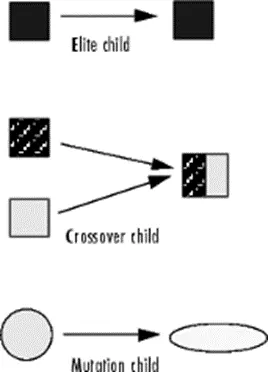
Mutation and Crossover explains how to specify the number of children of each type that the algorithm generates and the functions it uses to perform crossover and mutation.
The following sections explain how the algorithm creates crossover and mutation children.
Crossover Children
The algorithm creates crossover children by combining pairs of parents in the current population. At each coordinate of the child vector, the default crossover function randomly selects an entry, or gene, at the same coordinate from one of the two parents and assigns it to the child. For problems with linear constraints, the default crossover function creates the child as a random weighted average of the parents.
Mutation Children
The algorithm creates mutation children by randomly changing the genes of individual parents. By default, for unconstrained problems the algorithm adds a random vector from a Gaussian distribution to the parent. For bounded or linearly constrained problems, the child remains feasible.
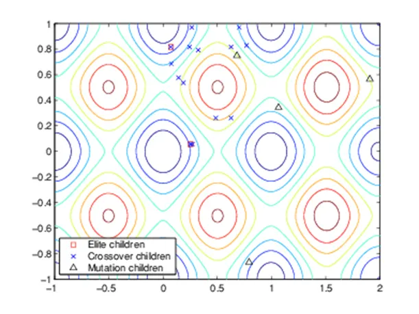
The following figure shows the children of the initial population, that is, the population at the second generation, and indicates whether they are elite, crossover, or mutation children.
The following figure shows the populations of later generations at iterations 60, 80, 95, and 100.
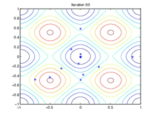
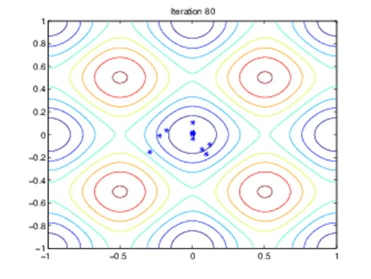
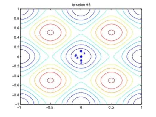
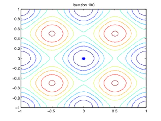
As the number of generations increases, the individuals in the population get closer together and approach the minimum point [0 0].
Stopping Conditions for the Algorithm
The genetic algorithm uses the following options to determine when to stop. See the default values for each option by running opts = optimoptions('ga').
- MaxGenerations: The algorithm stops when the number of generations reaches MaxGenerations.
- MaxTime: The algorithm stops after running for an amount of time in seconds equal to MaxTime.
- FitnessLimit: The algorithm stops when the value of the fitness function for the best point in the current population is less than or equal to FitnessLimit.
- MaxStallGenerations: The algorithm stops when the average relative change in the fitness function value over MaxStallGenerations is less than Function tolerance.
- MaxStallTime: The algorithm stops if there is no improvement in the objective function during an interval of time in seconds equal to MaxStallTime.
- FunctionTolerance: The algorithm runs until the average relative change in the fitness function value over MaxStallGenerations is less than Function tolerance.
- ConstraintTolerance: The ConstraintTolerance is not used as stopping criterion. It is used to determine the feasibility with respect to nonlinear constraints. Also, max(sqrt(eps), ConstraintTolerance) determines feasibility with respect to linear constraints.
The algorithm stops as soon as any one of these conditions is met.
Syntax for GA
- x = ga(fun,nvars) finds a local unconstrained minimum, x, to the objective function fun. nvarsis the dimension (number of design variables) of fun.
- x = ga(fun,nvars,A,b) finds a local minimum x to fun., subject to the linear inequalities A*x≤ b. ga evaluates the matrix product A*x as if x is transposed (A*x').
- x = ga(fun,nvars,A,b,Aeq,beq) finds a local minimum xto fun, subject to the linear equalities Aeq*x = beq and A*x ≤ b. (Set A=[] and b=[] if no linear inequalities exist.) ga evaluates the matrix product Aeq*x as if x is transposed (Aeq*x').
- x= ga(fun,nvars,A,b,Aeq,beq,lb,ub) defines a set of lower and upper bounds on the design variables, x, so that a solution is found in the range lb ≤ x ≤ ub. (Set Aeq=[] and beq=[] if no linear equalities exist.)
- x= ga(fun,nvars,A,b,Aeq,beq,lb,ub,nonlcon) subjects the minimization to the constraints defined in nonlcon. The function nonlcon accepts x and returns vectors C and Ceq, representing the nonlinear inequalities and equalities respectively. ga minimizes the fun such that C(x) ≤ 0 and Ceq(x) = 0. (Set lb=[] and ub=[] if no bounds exist.)
- x= ga(fun,nvars,A,b,Aeq,beq,lb,ub,nonlcon,options) minimizes with the default optimization parameters replaced by values in options. (Set nonlcon=[] if no nonlinear constraints exist.) Create options using optimoptions.
- x= ga(fun,nvars,A,b,Aeq,beq,lb,ub,nonlcon,intcon) or x = ga(fun,nvars,A,b,Aeq,beq,lb,ub,nonlcon,intcon,options) requires that the variables listed in intcon take integer values.
- x= ga(problem) finds the minimum for problem, a structure described in problem.
- [x,fval] = ga(___), for any previous input arguments, also returns fval, the value of the fitness function at x.
- [x,fval,exitflag,output] = ga(___)also returns exitflag, an integer identifying the reason the algorithm terminated, and output, a structure that contains output from each generation and other information about the performance of the algorithm.
- [x,fval,exitflag,output,population,scores] = ga(___)also returns a matrix population, whose rows are the final population, and a vector scores, the scores of the final population.
Objective: Objective of this project is to optimise the stalagmite function and find the global maxima of the function. By using GA solver, we can get minimum value. To get maximum, using GA solver, we will modify stalagmite function.
So the stalagmite function is-
`f(x,y)=f_1x*f_2x*f_1y*f_2y` ,.......(i) where
`f_1x=[sin(5.1pix+0.5)]^6`
`f_1y=[sin(5.1piy+0.5)]^6`
`f_2x=exp[-4ln(2)*(x-0.0667)^2/0.64]`
`f_2y=exp[-4ln(2)*(y-0.0667)^2/0.64]`
From equation (i) we will get minimum value , using GA solver. If we use negative sign then it will give maximum value through GA solver. So the equation will be
`f(x,y)=-(f_1x*f_2x*f_1y*f_2y)`
Function code for stalagmite will be
function [f] = stalagmite(input_vector);

f1x = (sin((5.1*pi*input_vector(1))+0.5))^6;
f1y = (sin((5.1*pi*input_vector(2))+0.5))^6;
f2x = exp((-4*log(2)*(input_vector(1)-0.0667)^2)/0.64);
f2y = exp((-4*log(2)*(input_vector(2)-0.0667)^2)/0.64);

f = -(f1x*f2x*f1y*f2y);
end
Here we will creat another function for stalagmite calculation that is
function [f]=get_stalagmite(x,y);
[xx yy]=meshgrid(x,y);

for i=1:length(xx);
    for j=1:length(yy);
        input_vector(1)=xx(i,j);
        input_vector(2)=yy(i,j);
        f(i,j)=stalagmite(input_vector);
    end
end
end
In this above 'get_stalagmite' function two 1D array(x,y) will be taken in optimization programme, basis on that 1D array 2D mesh(xx,yy) will be created using 'meshgrid' function.
Base upon that two 2D array(xx,yy) stalagmite function will be executed using two 'for' loop one another's inside.
Stydy-1: Now in optimization code first of all we will start with 'clear all', 'close all' & 'clc'. Then will creat two 1D array "x' & 'y' as mention before by using 'linspace' command where variable will rely in between 0 to 0.5 and number of variable will be 150.
Then will call the 'get_stalagmite' function for execution of 'stalagmite' function. Then we have to create another variable ‘num_cases’ and the value will be taken 50 and it will be number of iteration for the function.
Now optimization will be done using GA solver with a for loop where number of iteration will be 50, means stalagmite function will be optimized 50 times and here optimized values of ‘x’, ‘y’ and function ‘f’ will be ‘xopt’, ‘yopt’ and ‘fopt’ respectively.
We have to make sure ‘tic-toc’ function is using for time reading for optimization where ‘tic’ command should be just before the ‘for’ loop starting line and ‘toc’ command should be just after the end of ‘for’ loop.
Then We will create a 3D plot for stalagmite function using ‘surfc’ command where optimized values will also be shown. Through an adjacent subplot the graph of maximum value with respect to iteration will also be shown.
In case of study 1 inputes are not bounded. So the code will be
clear all
close all
clc

x=linspace(0,0.5,150);
y=linspace(0,0.5,150);
num_cases=50;

f=get_stalagmite(x,y);
tic
for i=1:num_cases;
    [input,fopt(i)]=ga(@stalagmite,2);
    xopt(i)=input(1);
    yopt(i)=input(2);

end
time_taken=toc
figure(1);
subplot(2,1,1);
hold on;
surfc(x,y,f);
shading interp;
plot3(xopt,yopt,fopt,'marker','o','markersize',5,'markerfacecolor','r')
xlabel('xopt')
ylabel('yopt')
zlabel('fopt')
title('Unbounded Inputs');
subplot(2,1,2)
plot(fopt)
xlabel('iteration')
ylabel('Function Maximum')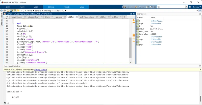
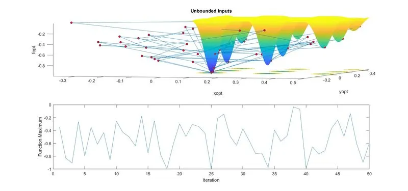
As the study 1 is unbounded and there are no constraints so the results are different in different run. As we can see from the plot the values of optimized function are all over the place as the sampling are random.
Stydy-2:
clear all
close all
clc

x=linspace(0,0.5,150);
y=linspace(0,0.5,150);
num_cases=50;
f=get_stalagmite(x,y);
tic
for i=1:num_cases;
    [input,fopt(i)]=ga(@stalagmite,2,[],[],[],[],[0;0],[0.5;0.5]);
    xopt(i)=input(1);
    yopt(i)=input(2);

end
time_taken=toc
figure(1);
subplot(2,1,1);
hold on;
surfc(x,y,f);
shading interp;
plot3(xopt,yopt,fopt,'marker','o','markersize',5,'markerfacecolor','r')
xlabel('xopt')
ylabel('yopt')
zlabel('fopt')
title('Bounded Inputs');
subplot(2,1,2)
plot(fopt)
xlabel('iteration')
ylabel('Function Maximum')
In study 2 we have given a lower bound (lb) of 0 and a upper bound (ub) of 0.5 for the function. rest of the coadding will remain same. results will be 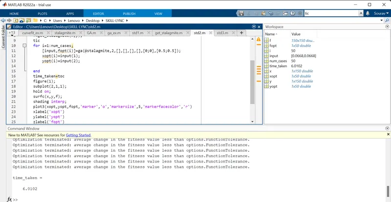
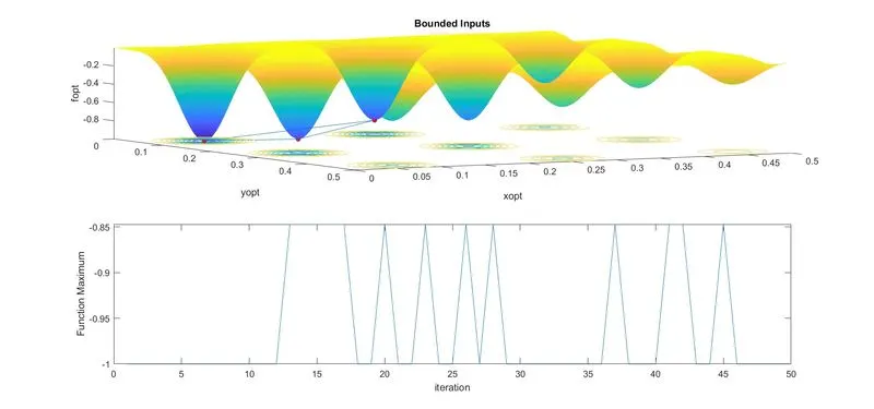
As we bounded the function in between 0 to 0.5 so the solutions are also in between 0 to 0.5. The result is better than study 1 but still many points in between bounded condition. To improve that we will go for study 3.
clear all
close all
clc
x=linspace(0,0.5,150);
y=linspace(0,0.5,150);
num_cases=50;
f=get_stalagmite(x,y);
options=optimoptions('ga');
options=optimoptions(options,'PopulationSize',180);
tic
for i=1:num_cases;
[input,fopt(i)]=ga(@stalagmite,2,[],[],[],[],[0;0],[0.5;0.5],[],[],options);
xopt(i)=input(1);
yopt(i)=input(2);
end
time_taken=toc
figure(1);
subplot(2,1,1);
hold on;
surfc(x,y,f);
shading interp;
plot3(xopt,yopt,fopt,'marker','o','markersize',5,'markerfacecolor','r')
xlabel('xopt');
ylabel('yopt');
zlabel('fopt');
title('Bounded Inputs with Population size 180');
subplot(2,1,2);
plot(fopt);
xlabel('iteration');
ylabel('Function Maximum');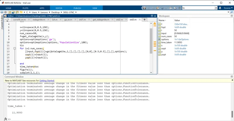
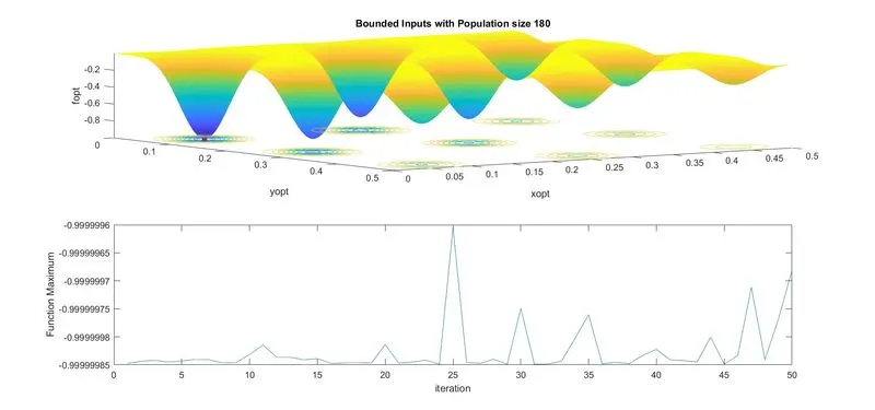
Hence we get the Global Maxima as we can see in the plot. But the time it takes almost double than study 2.
significance of running multiple iterations:
If we want to get more accurate value then we must run mutiple iterations. Multiple iteration refine the result.
References:
https://www.sciencedirect.com/topics/earth-and-planetary-sciences/stalactite
https://in.mathworks.com/help/gads/what-is-the-genetic-algorithm.html
https://in.mathworks.com/help/gads/how-the-genetic-algorithm-works.html