Project 2 - Rankine cycle Simulator
RANKINE CYCLE SIMULATOR
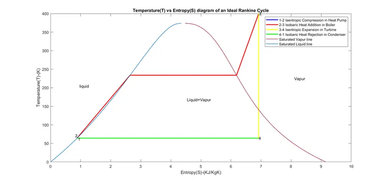
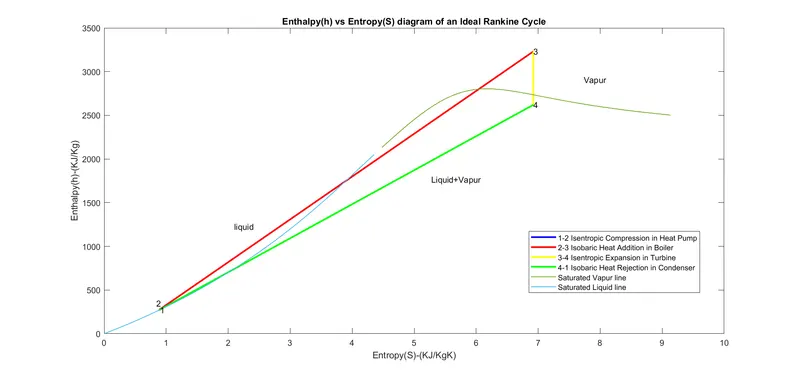
AIM:- Create a Ideal Rankine Cycle simulator using MATLAB where all importent data will be shown in command section. Also T-S diagram & H-S diagram will be ploted with proper labeling.
RANKINE CYCLE:- The Rankine cycle or Rankine Vapor Power Cycle is the process widely used by power plants such as coal-fired power plants or nuclear reactors. In this mechanism, a fuel is used to produce heat within a boiler, converting water into steam which then expands through a turbine producing useful work.
The steps in the Rankine Cycle as shown in below figure and the corresponding steps in the Temperature vs Entropy diagram (2nd figure) are outlined below:
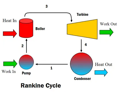
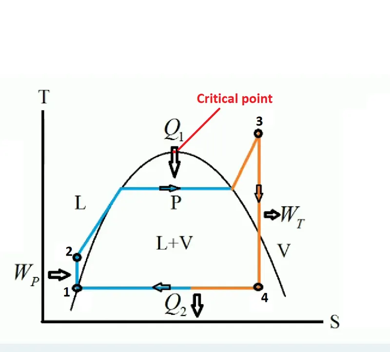
1-2 Isentropic Compression. The pressure of the condensate is raised in the feed pump. Because of the low specific volume of liquids, the pump work is relatively small and often neglected in thermodynamic calculations.
2-3 Isobaric Heat Transfer. High pressure liquid enters the boiler from the feed pump and is heated to the saturation temperature. Further addition of energy causes evaporation of the liquid until it is fully converted to saturated steam.
3-4 Isentropic Expansion. The vapor is expanded in the turbine, thus producing work which may be converted to electricity. In practice, the expansion is limited by the temperature of the cooling medium and by the erosion of the turbine blades by liquid entrainment in the vapor stream as the process moves further into the two-phase region. Exit vapor qualities should be greater than 90%.
4-1 Isobaric Heat Rejection. The vapor-liquid mixture leaving the turbine (4) is condensed at low pressure, usually in a surface condenser using cooling water. In well designed and maintained condensers, the pressure of the vapor is well below atmospheric pressure, approaching the saturation pressure of the operating fluid at the cooling water temperature.
As we are dealing with Ideal Rankine Cycle in this project so there are some assumptions.
1. The cycle does not involve any friction. Therefore, the working fluid does not experience any pressure drop as it flowes in pipes or devices such as heat exchangers etc.
2. All Expansion and compression process take place in a quasiequilibrium manner.
3. The pipes containing the various components of a system are well insulated, and heat transfer through them is negligible.
4. All devices are steady flow devices, where change in kinatic energy and change in potaintial energy are neglated.
Assuming these(above) 4 conditions heat addition in boiler, pump work, turbine work done, net work done, net efficiency and stam flow rate will be calculated using steady flow energy equation.
So according to steady flow energy equation total energy input will be equal to total energy output of system.
`in`in = `in`out
`q`in + `h`in + `w`in + `Kin`in + `P in`in = `q`out + `h`out + `w`out + `Kin`out + `P in`out
Neglating Kinetic energy & potaintial energy we will get-
`q`in + `h`in + `w`in = `q`out + `h`out + `w`out .......(1)
Applying eqn no (1) to 1-2 Isentropic Compression we will get-
`h1+wp=h2` [where `q`in = `q`out = `w`out = 0]
so Pump Work wp=h2-h1
Applying eqn no (1) to 2-3 Isobaric Heat Transfer we will get-
q1+h2=h3 [where `w`in = `w`out = `q`out = 0]
so heat addition to boiler q1=h3-h2
Applying eqn no (1) to 3-4 Isentropic Expansion we will get-
h3=h4+wt [where `q`in = `q`out = `w`in = 0]
so work done by turbine wt=h3-h4
Net work done(Wnet)=wt-wp
rankine cycle efficiency(`eta`)=`(wt-wp)/(q1)`
CODE:
We will start the code by a hade line 'Rankine Cycle Simulator' using 'fprintf' command. Then mentaion all 4 process using again 'fprintf' command. we have to make sure that they are in different line using '\n'. Then we will create three proper named variable those will contain mentaion inputs in problem using 'input' command. Next we will create proper named variables for all four state points containing Pressure,Temperature, Entropy & Enthalpy values.
After that we have to create a 'for' loop where Entropy and Enthalpy values will be calculated for a set of Temperature values. These values will create Saturated dome.
Then Turbine Work Done, Pump Work, Heat Addition in Boiler, Net Work, Efficiency & Steam Flow Rate will be calculated and stored in a proper named variable. Then using 'fprintf' comand all the variables of 4 points will be displayed in 'command window'.
At last two plots(T-S diagram & H-S diagram) will be created using 'plot' comand with proper labeling and legends.
So the final code will be-
close all
clear all
clc

% Rankine Cycle Simulator
fprintf('%50fRankin Cycle Simulator\n','')
%Process Description
fprintf('1-2 Isentropic Compression in Heat Pump\n')
fprintf('2-3 Isobaric Heat Addition in Boiler\n')
fprintf('3-4 Isentropic Expansion in Turbine\n')
fprintf('4-1 Isobaric Heat Rejection in Condenser\n')

%Inputs
p3=input('Pressure(in Bar) of Turbine Inlet is:')
t3=input('Temperature(in Celsius) of Turbine Inlet is:')
p4=input('Pressure(in Bar) of Turbine Outlet is:')
%state 3
h3=XSteam('h_pT',p3,t3);
s3=XSteam('s_pT',p3,t3);

%state 4
s4=s3;
g=1.4;
t4=t3*((p4/p3)^(1-(1/g)));
h4=XSteam('h_pT',p4,t4);

%stage 1
t1=t4;
p1=p4;
h1=XSteam('hL_T',t1);
s1=XSteam('sL_T',t1);

%stage 2
s2=s1;
p2=p3;
t2=XSteam('T_ps',p2,s2);
h2=XSteam('h_pT',p2,t2);

%saturated liquid and steam points inbetween 2-3
t21=XSteam('Tsat_p',p2);
t22=XSteam('Tsat_p',p2);
s21=XSteam('sL_T',t21);
s22=XSteam('sV_T',t22);
h21=XSteam('hL_T',t21);
h22=XSteam('hV_T',t22);

%saturation dome
temp=linspace(0,900,1000);
for i=1:length(temp);
    sv(i)=XSteam('sV_T',temp(i));
    sl(i)=XSteam('sL_T',temp(i));

    hv(i)=XSteam('hV_T',temp(i));
    hl(i)=XSteam('hL_T',temp(i));
end


 WT=h3-h4;%turbine workdone
 WP=h2-h1;%pump work
 Wnet=WT-WP;%net work
 qs=h3-h2;%heat addition
 n_per=(Wnet/qs)*100;%Efficiency
 stm_rate=3600/(WT-WP);%steam rate per second
 Back_work_ratio=WP/WT;%Back work ratio

 fprintf('At Point 1:\nPressure(P1)=%f Bar\nEntropy(S1)=%f KJ/KgK\nEnthalpy(H1)=%f KJ/Kg\nTemperature(T1)=%f Degree Celcius\n',p1,s1,h1,t1)
 fprintf('At Point 2:\nPressure(P2)=%f Bar\nEntropy(S2)=%f KJ/KgK\nEnthalpy(H2)=%f KJ/Kg\nTemperature(T2)=%f Degree Celcius\n',p2,s2,h2,t2)
 fprintf('At Point 3:\nPressure(P3)=%f Bar\nEntropy(S3)=%f KJ/KgK\nEnthalpy(H3)=%f KJ/Kg\nTemperature(T3)=%f Degree Celcius\n',p3,s3,h3,t3)
 fprintf('At Point 4:\nPressure(P4)=%f Bar\nEntropy(S4)=%f KJ/KgK\nEnthalpy(H4)=%f KJ/Kg\nTemperature(T4)=%f Degree Celcius\n\n',p4,s4,h4,t4)
 fprintf('Work Done by Turbine(WT)=%f KJ/Kg\nWork Done by Pump(WP)=%f KJ/Kg\nNet Work Done(Wnet)=%f KJ/Kg\nHeat Addition in Boiler(qs)=%f KJ/Kg\nEfficiency(n_per)=%f Percent\nSpecific Steam Consumption(SSC)=%f Kg/KWh\nBack Work Ratio=%f \n',WT,WP,Wnet,qs,n_per,stm_rate,Back_work_ratio)

 figure(1)
 plot([s1 s2],[t1 t2],'color','blue','LineWidth',2)
 hold on
 plot([s2 s21],[t2 t21],[s21 s22],[t21 t22],[s22 s3],[t22 t3],'Color','red','LineWidth',2)
 plot([s3 s4],[t3 t4],'Color','yellow','LineWidth',2)
 plot([s4 s1],[t4 t1],'Color','green','LineWidth',2)
 plot(sv,temp,'LineWidth',1)
 plot(sl,temp,'LineWidth',1)
 gtext('1')
 gtext('2')
 text(s3,t3,'3')
 text(s4,t4,'4')
 gtext('liquid')
 gtext('Vapur')
 gtext('Liquid+Vapur')
 legend('1-2 Isentropic Compression in Heat Pump','2-3 Isobaric Heat Addition in Boiler','','','3-4 Isentropic Expansion in Turbine','4-1 Isobaric Heat Rejection in Condenser','Saturated Vapur line','Saturated Liquid line')
 xlabel('Entropy(S)-(KJ/KgK)')
 ylabel('Temperature(T)-(K)')
 title('Temperature(T) vs Entropy(S) diagram of an Ideal Rankine Cycle')

 figure(2)
  plot([s1 s2],[h1 h2],'color','blue','LineWidth',2)
 hold on
 plot([s2 s3],[h2 h3],'Color','red','LineWidth',2)
 plot([s3 s4],[h3 h4],'Color','yellow','LineWidth',2)
 plot([s4 s1],[h4 h1],'Color','green','LineWidth',2)
 plot(sv,hv,'LineWidth',1)
 plot(sl,hl,'LineWidth',1)
 gtext('1')
 gtext('2')
 text(s3,h3,'3')
 text(s4,h4,'4')
 gtext('liquid')
 gtext('Vapur')
 gtext('Liquid+Vapur')
 legend('1-2 Isentropic Compression in Heat Pump','2-3 Isobaric Heat Addition in Boiler','3-4 Isentropic Expansion in Turbine','4-1 Isobaric Heat Rejection in Condenser','Saturated Vapur line','Saturated Liquid line')
 xlabel('Entropy(S)-(KJ/KgK)')
 ylabel('Enthalpy(h)-(KJ/Kg)')
 title('Enthalpy(h) vs Entropy(S) diagram of an Ideal Rankine Cycle')
Here are the diagrams-
T-S Diagram:
H-S Diagram:
COMMAND WINDOW:
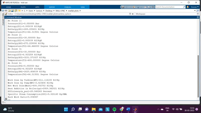
So, Net Work Done is 608.092782 KJ/Kg
Back Work Ratio is 0.004947
REFERANCE:
https://thermopedia.com/content/1072