External flow simulation over an Ahmed body using Fluent

OBJECTIVE:

Simulation of External flow over the Ahmed body is conducted in this challenge. Parameters such as coefficient of lift and coefficient of drag are estimated and validated. The wake region is investigated. The Grid Independence test is conducted.

SOFTWARES USED:

1. Ansys Fluent 2021 R1

AHMED BODY AND ITS SIGNIFICANCE:

The Ahmed body is a geometric entity that represents a standard passenger car. The geometry was first proposed by Ahmed and Ramm in 1984 and was extensively used to study the effects of the geometry on the wake region. Over the years, numerous studies have been conducted on the Ahmed body both computationally and experimentally using wind tunnels. Since a lot of data is available on the Ahmed body, today the geometry is primarily as a validation tool for CFD codes. The geometry of the Ahmed body is shown below:

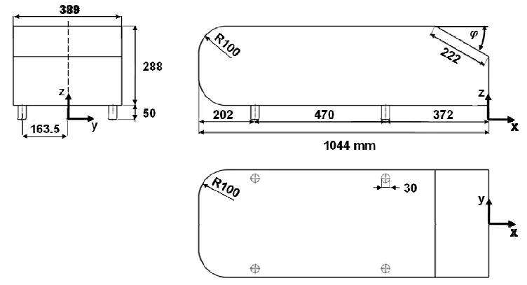
Variation of the slant angle (`psi`) at the back of the geometry is the primary parameter in the characterization of the wake region. It has been found out that `psi` = 30 deg is the critical value of slant angle. For Ahmed bodies, whose `psi` is below 30 deg, a pair of counter-rotating vortices is generated. These vortices help in preventing the separation of flow along the slant surface. Above a `psi` of 30, separation of flow occurs somewhere along the slant, and flow develops into a relatively larger recirculating region in the wake.

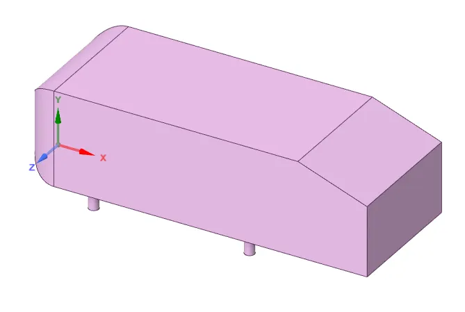
In this challenge, the study is performed on the Ahmed body whose slant angle is 20 degrees using Ansys fluent. The freestream speed of flow is taken as 25 m/s and the fluid is 'air'. The wake region is analyzed with contours and vector plots of velocity at certain probe locations behind the geometry. Parameters such as coefficient of lift, coefficient of drag, and point of separation of flow are estimated. Shown below is the CAD Model of the Ahmed body used in the challenge.

CASE SETUP IN ANSYS FLUENT:

• Since the Ahmed body is symmetric about the X-Y plane (shown above), the body is to be split into two symmetric half and the 'symmetry' boundary condition is to be applied. This helps to save a lot of computational cells that can be used to further refine the wake region.
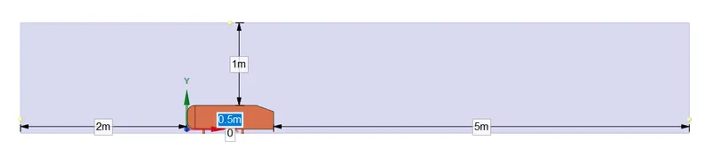
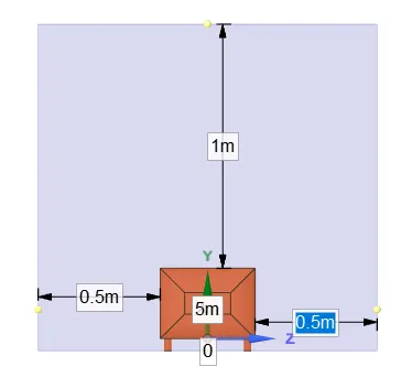
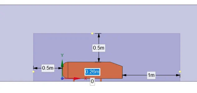
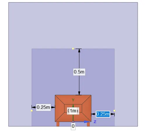
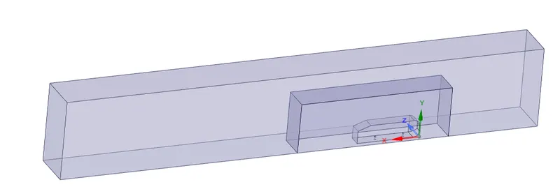
• The given problem is external aerodynamic simulation. A wind tunnel is created over the Ahmed body using the 'Enclosure' option in Spaceclaim. This outer enclosure contains a smaller, inner enclosure (for local refinement) which in turn contains the surface of the Ahmed body. While creating the enclosures, the 'Interference' option was used to remove any geometric interference and common regions created by the double enclosures. The 'topology' option is set to 'Share' to ensure data is shared between different enclosures. The dimensions of the enclosure are shown:

Outer Enclosure and Inner Enclosure:

• The outer enclosure is of bigger dimensions to make the inflow and outflow boundary conditions not be influenced by the presence of the Ahmed body. But it is impractical to make the whole domain thoroughly refined because it would result in a waste of computational resources. Hence a smaller inner enclosure is created for the purpose of local refinement. It is of immense importance to refine the mesh much more, closer to the geometry, and is shown below.

• Shown below is the final geometry that is to be used for meshing. Note that the 'split body' command has already been used on the geometry.

• 
  
  

• Next, the mesh module is opened. Since the geometry of the outer enclosure is made of straight lines, the 'hex' mesh is used. The inner enclosure holds the surface of the Ahmed body and hence is 'triangle dominant'. The 'Multizone' mesh method is applied to the outer enclosure to connect between different mesh types. The base mesh size is set to 0.1 meters.
• The inner enclosure is given 'mesh body sizing' and is set to a size of 0.03 meters. Mesh 'face sizing' with a size of 0.004 meters is given on the cylindrical stands of the Ahmed body to prevent geometry distortion at the stands. To capture the near-wall physics accurately, a boundary layer mesh (Body fitted Mesh) (or) Mesh inflation is provided to the geometry. To come up with the right mesh size, the following calculations are done. Shown below is the mesh obtained.

• To capture the near-wall effects, the `k-omega` SST Turbulence model (y+ range 1 to 5) is preferred. The mesh inflation option is set to 'Total thickness'. Two parameters are required: The total thickness of inflation and the number of inflation layers. Firstly, the boundary layer thickness at the end of the Ahmed body is calculated using the boundary layer formula for turbulent flow over a flat plate. Considering the y+ for the problem as 5, the first layer thickness is calculated. Now, the number of inflation layers can be calculated using Sum of n terms of the GP formula.

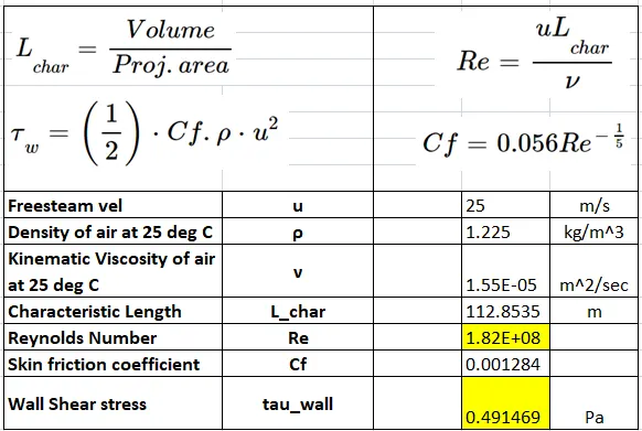
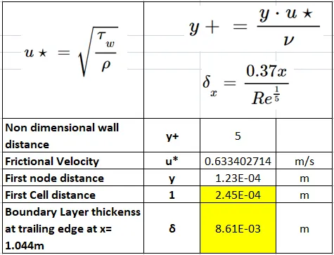
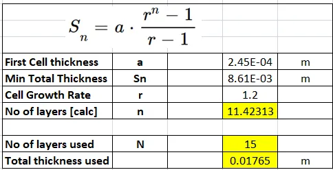
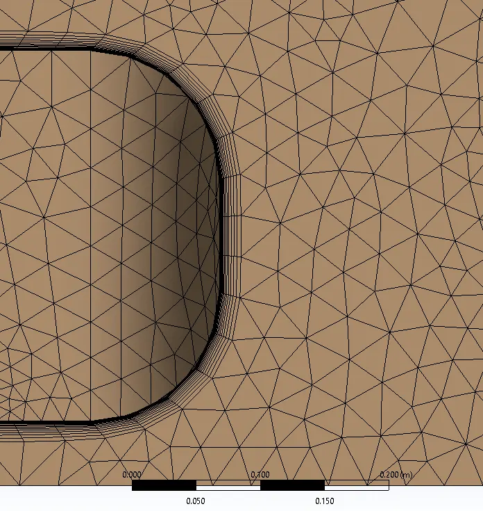
• The number of inflation layers is ~12. Taking into account the slanted surface at the end of the geometry and the developing vortices, the number of layers is set to 15 with a total inflation thickness of 0.01766 meters. With this, the meshing is complete. The inflation layers are shown below.

• Next, Fluent is opened and a mesh-check is performed. A pressure-based steady-solver is used for the case as the flow speed of 25 m/s is well below Mach 0.3. At the reference values, the projected area, length, velocity, region from which flow occurs are specified. The turbulence model is set to `k-omega` SST. Material is 'air'. The boundary conditions are specified next.

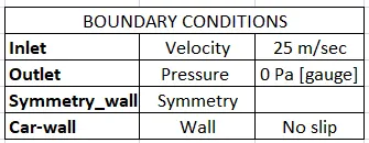
• The problem is then initialized using the Hybrid solver. Plots such as coefficient of lift, coefficient of drag, wall shear stress, pressure contours, velocity contours, vector plots are set up before the simulation. Finally, the case is run for 500 iterations.

RESULTS:

A) Convergence:

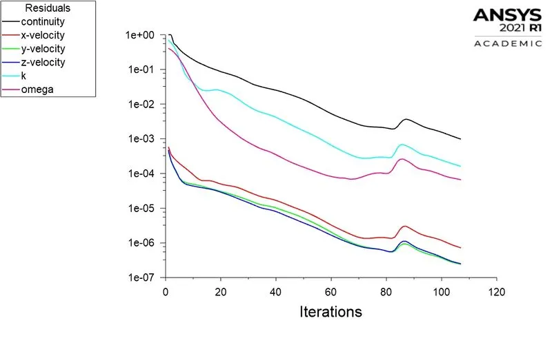
1. The number of iterations was set to 500.
2. But it is observed that the residuals have fallen below the specified tolerances and the solution attains convergence in ~110 iterations.

B) Coefficient of Drag and Coefficient of Lift:

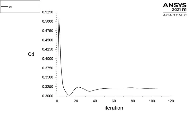
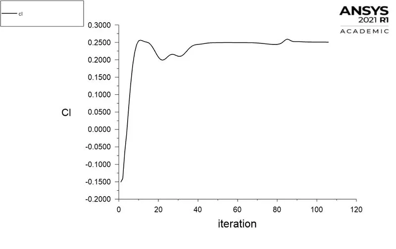
1. The formation of the low-pressure wake region dictates how high is the drag coefficient. The steady-state drag coefficient is found to be 0.32096. This result can be validated from [3] with an error of 7.34%.
2. The formation of vortices in the wake results in the lift. The steady-state lift coefficient is found to be 0.2504.

C) Wall shear stress and the Point of separation:

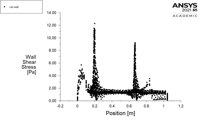
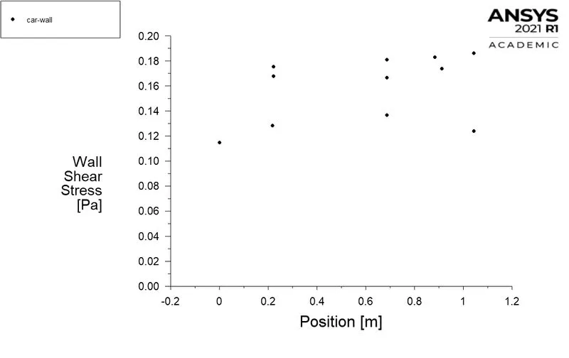
1. Boundary layer separation occurs when there is an adverse pressure gradient and zero normal velocity gradient at the wall (i.e zero wall shear stress) simultaneously. The possibility of this occurring in the Ahmed body is at the slant surface.
2. But, from literature, it is known that the flow does not separate at slant angles less than 30.
3. The LHS plot is the wall shear stress plot along the entire length of the Ahmed body. The plot on the RHS is the zoomed-in range of the wall shear stress close to zero ranging from 0.0 Pa to 0.2 Pa.
4. The result obtained is in accordance with the literature. The minimum wall shear stress obtained along the surface of the entire surface is always greater than 0.1.
5. However, the flow separation occurs right at the end of the slant surface at the rear of the geometry. This flow separation results in a recirculation region of low pressure and determines the coefficient of drag of the body.

D) X-Y Contours of Pressure and Velocity:

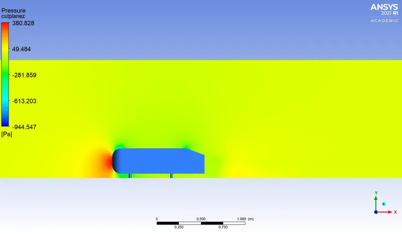
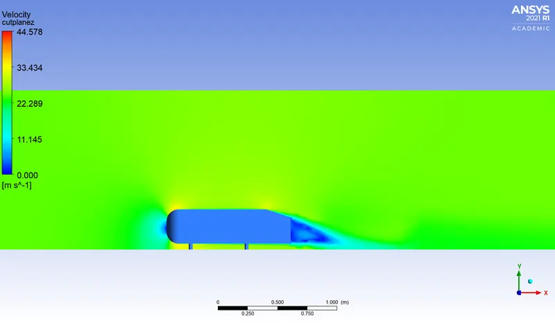
1. The contours are generated on an X-Y plane at Z = 0.
2. Just behind the slanted surface of the Ahmed body, a recirculation region is formed. This will be demonstrated more clearly by the vector plots in the coming section. The recirculation region has a lower pressure core and is represented by the light green patches in the contour. The scale defined in the contour represents the gauge pressure and hence shows negative pressure values at the recirculation region.
3. The pressure is maximum at the leading boundary of the Ahmed body because the flow is stagnated here. Also, at points where there exists curvature such as the filleted region at the leading boundary and the sharp beginning of the slant, there exist local low-pressure regions due to a sudden change in the geometry.
4. The velocity contour shows the flow over the slanted region. The flow does separate till the end of the slanted surface, after which separation occurs. A low-velocity region is formed at the recirculation region. This low-pressure region extends far into the wake of the car along with the formation of counter-rotating vortices that is shown in the next section.
5. At the different curvatures on the surface of the Ahmed body, where local low pressure exists, the regions have relatively higher velocities.

E) Streamline and Vector Plots:

a) Streamline: The Ahmed body is colored by the pressure and the streamlines are colored by velocity.

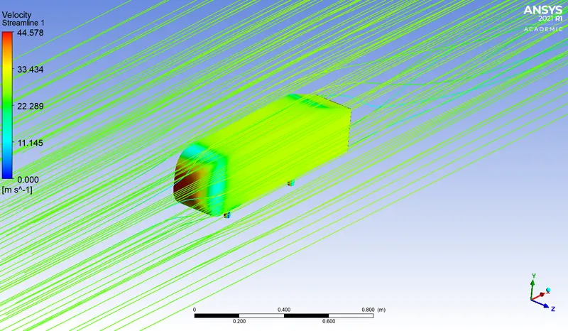
b) Vector plot of Velocity:

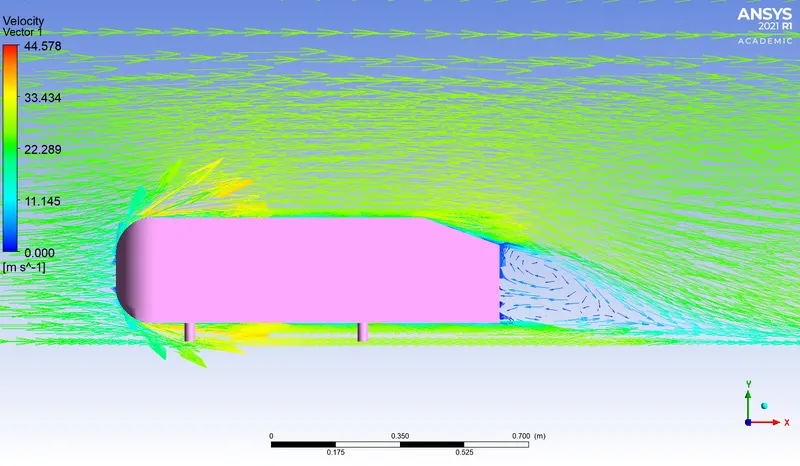
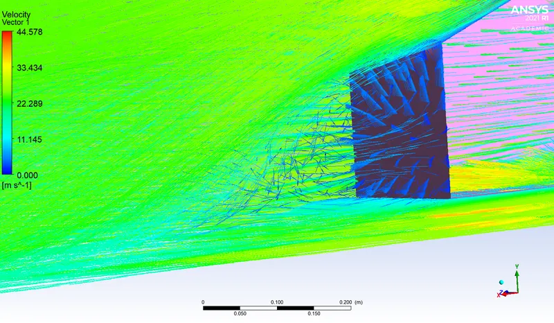
1. The vector plot shows the direction of flow at all locations. It is colored by velocity. The recirculation region is clearly seen from the images shown above.
2. This recirculation region further develops into a pair of counter-rotating trailing vortices that have a low-pressure region in the core. These vortices are visualized better in the next section.

c) Vector plots at Y-Z Plane probes:

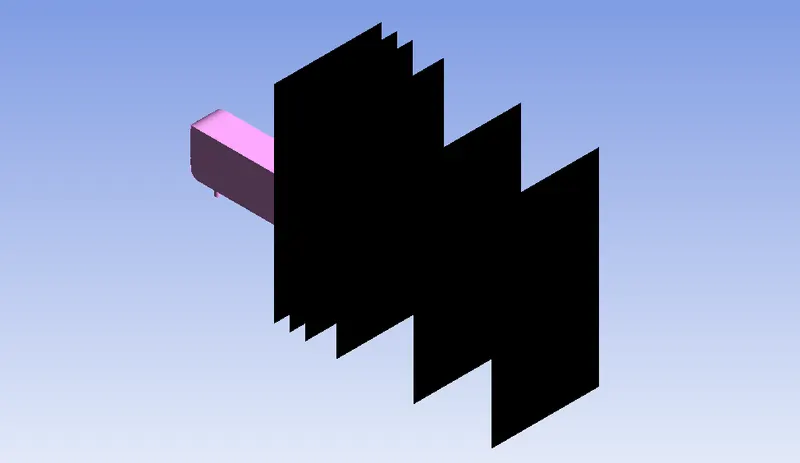
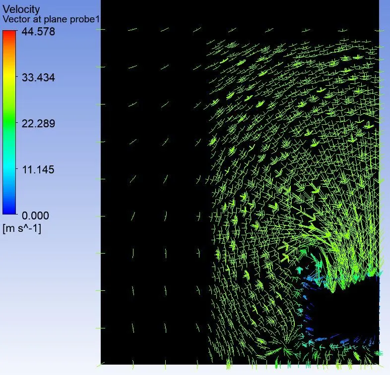
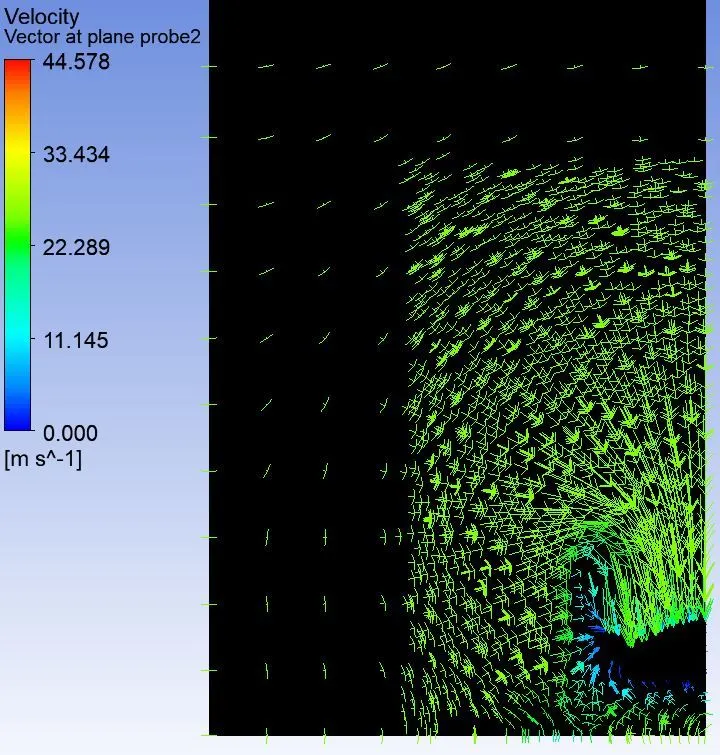
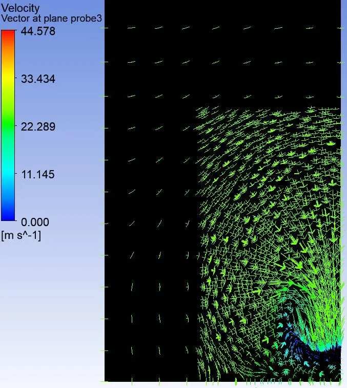
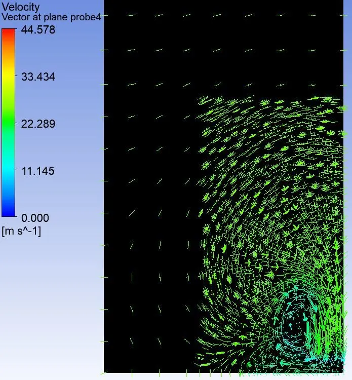
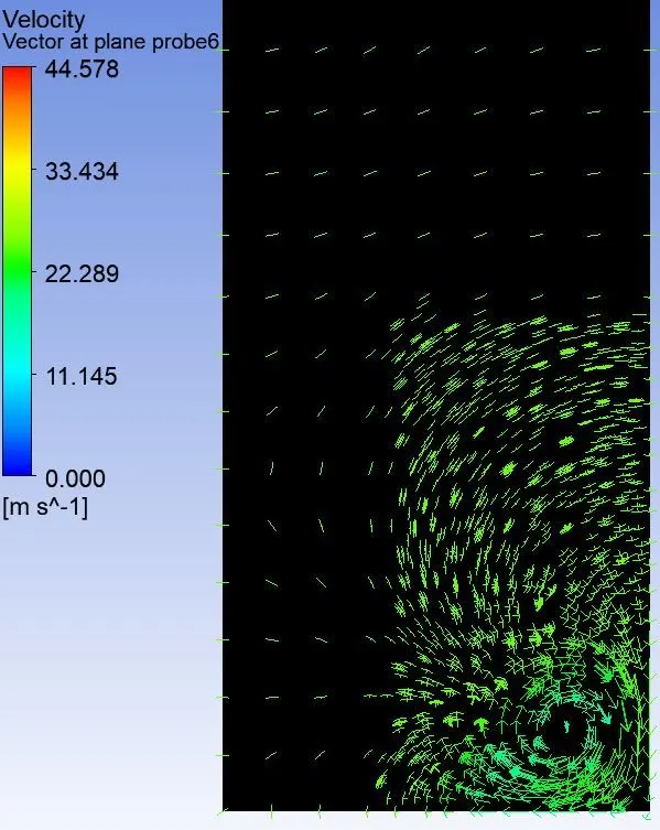
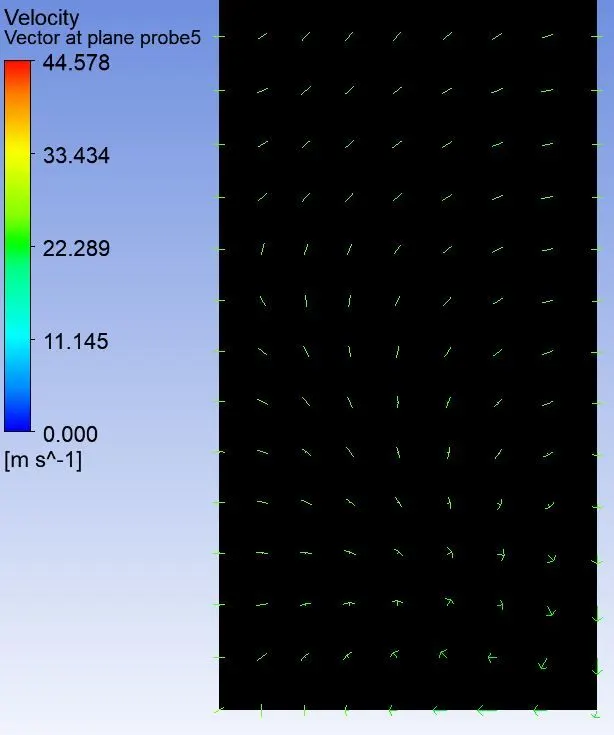
1. These vector plots are generated at specific Y-Z plane probes as shown above at distances 1.1m, 1.2m, 1.3m, 1.5m, 2m, 2.5m respectively from the origin. The Origin is located at the front end of the Ahmed body.
2. It is observed that with increasing distance in the wake, the vortices become fully developed. The distance up to which the vortices influence the wake is slightly above 2 meters.
3. It is to be noted that the images shown above represent only one vortex as the geometry was split and symmetry BC was applied. Hence, it can be assumed that a similar vortex is formed on the right-hand side of the displayed vortex.
4. Eventually, the wake dies out and the flow is reattached. At a distance of 2.5 meters, it is observed that the flow is the usual freestream flow.

F) Velocity Profile at various Line probes:

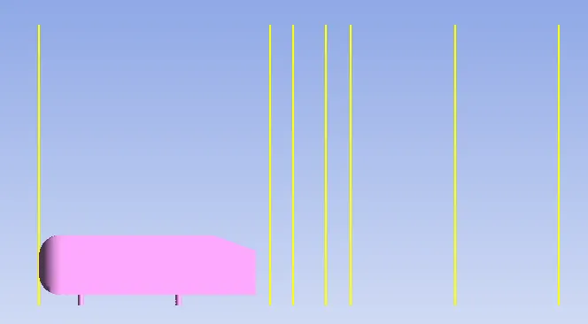
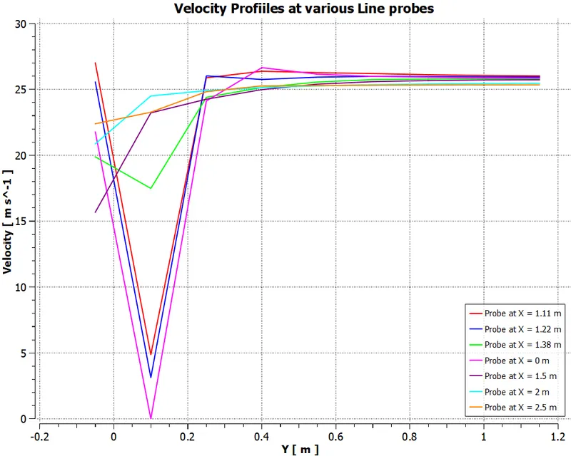
1. Various line probes are drawn at distances of 1.11 m, 1.22 m, 1.38 m, 0 m, 1.5 m, 2 m, 2.5 m respectively from the origin. The Origin is located at the front end of the Ahmed body.
2. The velocity profile is drawn at each of these lines probes wrt the distance in the Y direction.
3. For the first three probes, the velocity reduces from the freestream speed to a minimum at the recirculation region and climbs steadily up to a value after which the influence of the wake is not present. From here, the gradient in the velocity is very small and it attains the free stream speed. For the probe at X=0, the flow reduces from freestream to 0 at the stagnation point and then follows the same trend as before.
4. The rest of the probes that are present in the influence of the wake, have velocities lesser than the freestream speed and gradually rise to the freestream speed. No points of minimum speed are observed at these probes.

G) Grid Independence Test:

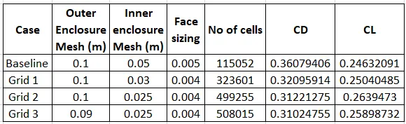
The case is set up using meshes of increasing local refinement in an attempt to get mesh-independent results. The following are the results obtained for the combination of different mesh sizes. The maximum number of cells that can be used in the academic version of fluent is 512000 cells.

The coefficient of drag attains a consistent value up to the 2nd decimal place in grid 2 and grid 3. Grid 3 holds the maximum refinement and the cell count is close to the maximum value. The error in the drag coefficient obtained using grid 3 with reference to [3] is 3.76%. Grid 2 produces an error of 4.41%. Hence, grid 3 and grid 4, both produce close values and both these results can be considered grid-independent. The results obtained in the other sections of the challenge are based on Grid 1. The meshes are shown below:

Baseline mesh:

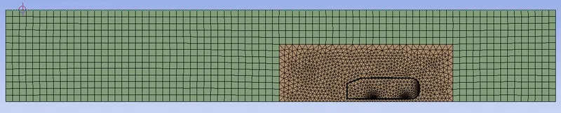
Grid 1:

Grid 2:

Grid 3:

CONCLUSION:

The flow over the Ahmed body is conducted and the wake region is visualized using Vector and Contour plots and analyzed. The coefficient of drag and coefficient of lift is estimated. The point of separation and its influence is talked upon. The grid Independence test is conducted.

References:

[1]: Experiments and numerical simulations on the aerodynamics of the Ahmed body, W. Meile, G. Brenn, A. Reppenhagen, B. Lechner, A. Fuchs

[2]: Flow and Turbulence Structures in the Wake of a Simplified Car Model (Ahmed Model), H. Lienhart, C. Stoots, S. Becker

[3]: Aerodynamic Study of an Ahmed body with the help of CFD Simulation, Indrashis Saha, Tathagatha Mukherjee