Parametric study on Gate valve using Fluent

OBJECTIVE:

To perform a parametric study on the lift of a gate valve wrt the % in Gate Opening using Ansys Fluent.

SOFTWARE USED:

1. Ansys Fluent 2021 R1

GEOMETRY AND PHYSICAL MODEL:

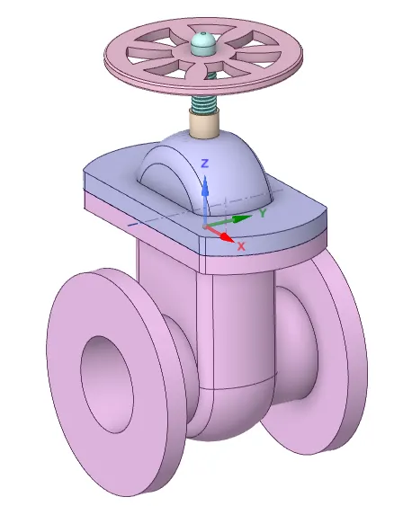
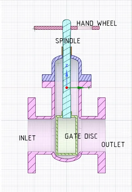
A Gate Valve is a hydraulic component that gives an outlet mass flow rate proportional to the opening of a gate present in it. Shown below is the geometry of the Gate Valve. It consists of a Gate Disc which blocks the incoming flow. The position of the gate disc is adjusted using a spindle and a hand-wheel system thereby adjusting the % of the opening.

In this challenge, the Mass flow rate (MFR) is the desired parameter that is to be studied wrt different opening heights of the gate disc. This problem can be simulated in a conventional way, but it becomes a tedious job to adjust the geometry in Spaceclaim for every lift, update mesh and open fluent to run the case to check the output MFR. In such situations, the Parametric study is used. The Gate disc lift is specified as a parameter in SpaceClaim. If any input is specified as a parameter, a Parameters tab gets added to Ansys Workbench. The parameter settings can be accessed from this tab. The input parameters are entered here directly without the need of opening any other modules of Ansys. Each new value of the input parameter is denoted as a Design Point. A one-time specification of the list of the input parameters and the output parameters that are needed must be done. Ansys then solves the complete Design Cases including the updation of fluid volume according to the change in the geometry, the meshing, and calculation of the solution without having to open any module. The complete results are displayed in the Design Point Table.

In this challenge, the opening of the Gate disc is varied from 10% to 80%, and the MFR is calculated in every case. The Flow Coefficient and the Flow Factors are estimated in every case. In order to avoid the extensive, conventional method of modifying the inputs each time, the Parametric method is used. The % Opening is provided as the Input parameter and the MFR, Flow Coefficient, and Flow Factor are provided as the output parameters.

CASE SETUP IN ANSYS:

I) Geometry:

The STEP geometry is imported in Spaceclaim. The inlet fluid length and the exit fluid length are extended to 800 mm in order to obtain a steady value of flow parameters at the inlet and outlet C/S without being influenced by the Gate Valve. The geometry is shown below.

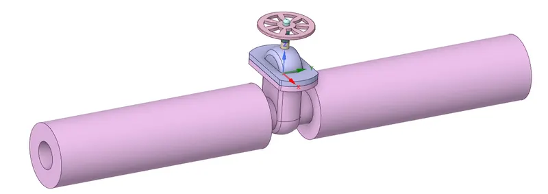
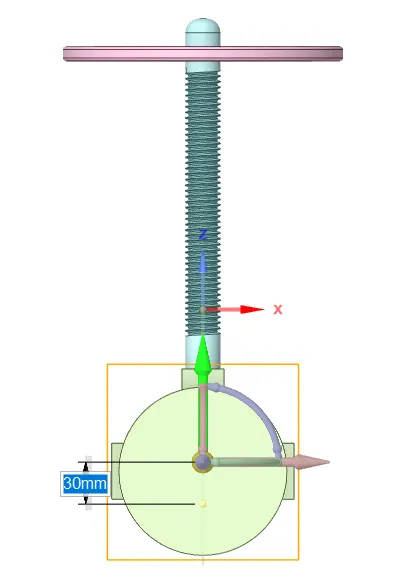
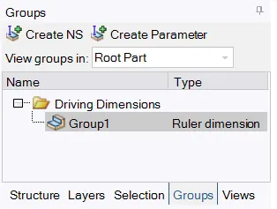
Next, the % Gate opening is specified as a parameter by doing the following: The 'Move' command is used on the Gate disc. The axis of movement is selected and the gate valve is moved manually up to the required distance, for say 10% opening, 5.05 mm. Now, on the LHS in the design tree window, navigate to the Groups tab. Here, the 'Create Parameter' is clicked to create a group parameter. The created group parameter represents the height of the lift.

==>

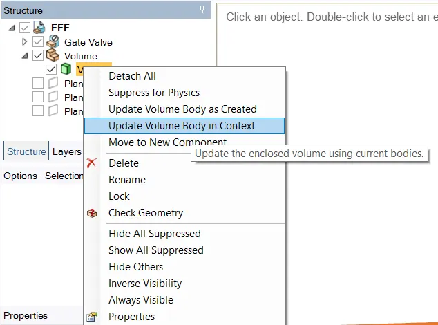
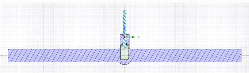
Next, the fluid volume is extracted using the 'Extract Volume' option. To make sure that changes in the geometry get reflected onto the fluid volume, the fluid volume is right-clicked on the design tree and the 'Update Volume body in context' option is selected. Now, to view the updated fluid volume, a cross-sectional view is generated and checked as well. The fluid volume and the cross-section of the updated geometry are shown below.

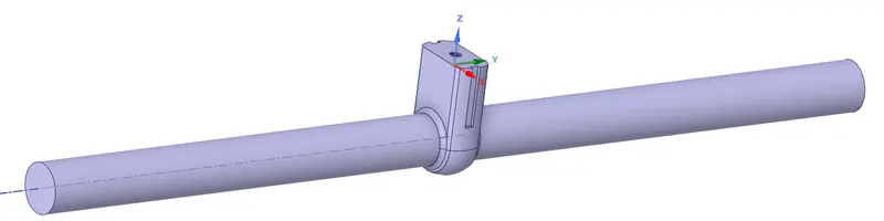
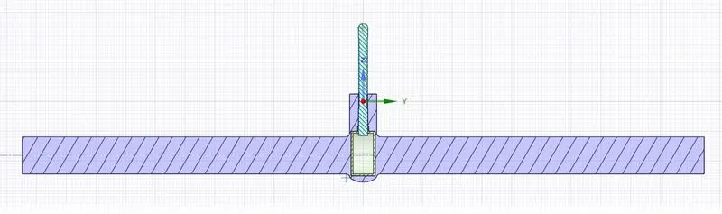
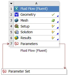
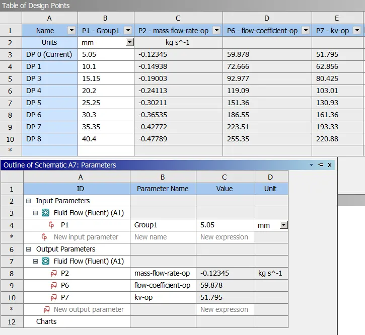
Now, the user can exit SpaceClaim. A new 'Parameters' option will now be visible on Workbench as shown below. Double-clicking the parameters button will take the user to a new window in Workbench that displays all the Input and Output parameters and a table of Design Points.

==>

II) Meshing:

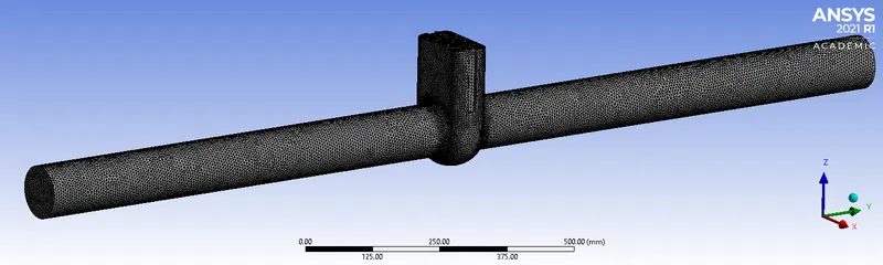
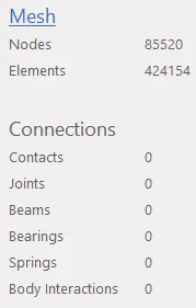
A regular Tetrahedral mesh is specified. The element size is specified as 6 mm. Named selections Inlet and Outlet are made. The 'Element Quality' mesh metric is set up.

III) Fluent set-up:

• A pressure-based, steady-state solver is used. Gravity is enabled with -9.81 m/s^2 in the Z direction as per the orientation.
• The flow is found to be turbulent from the Reynolds number. Hence, the Realizable k-epsilon` with Scalable Wall function turbulence model is enabled.
• 'Air' is deleted from the fluid domain and 'Water' is added.
• A pressure inlet boundary condition is specified. Inlet pressure of 10 Pa (gauge) is specified. The outlet pressure is 1 atm.
• The solution is initialized using the Standard solver.
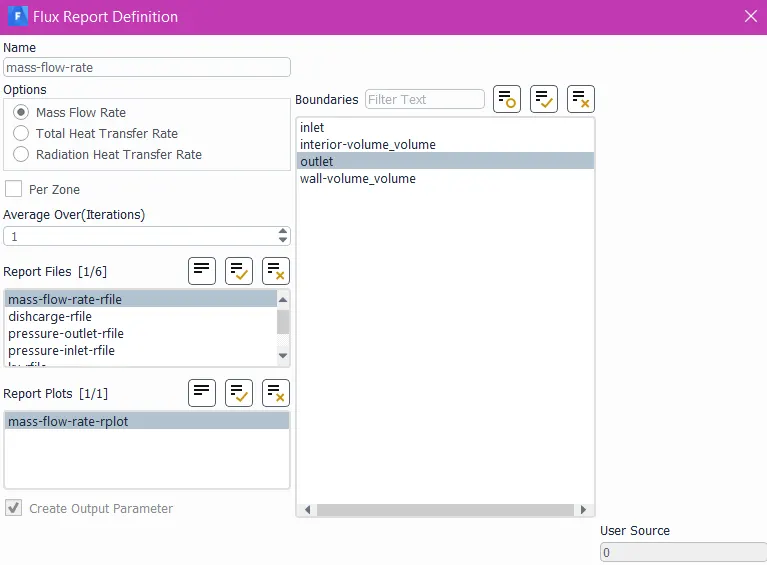
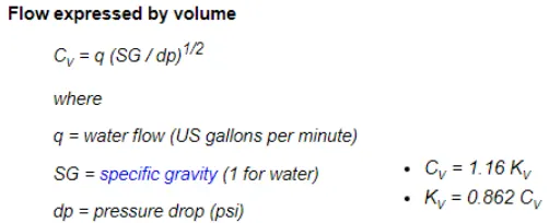
• Next, report definitions for Static Pressure inlet, Static Pressure outlet, Mass flow rate, Volume flow rate are specified. To create an 'Output Parameter' for the Parametric study, the checkbox 'Create Output Parameter' is ticked. In this challenge, the MFR, Flow Coefficient, and Flow Factor are specified as parameters. Flow coefficient and Flow factor are calculated using user-defined expressions of area-averaged flow. The expressions are shown below.

• The 'Coupled' scheme is used for Pressure-Velocity Coupling.
• Lastly, the number of iterations is set to 250 and the case is run.
• After the case runs successfully, Fluent is closed and the 'Parameters' tab is opened to add additional Design Points.
• The maximum valve lift is found from Spaceclaim as 50.5 mm. Hence using this value, % openings are defined ranging from 10% to 80% as Design Points. The input parameters are entered in the Design Table.

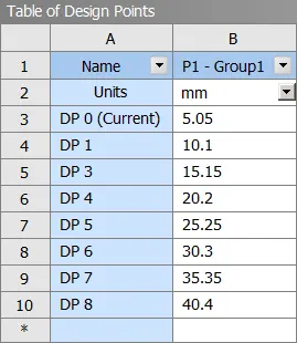
• The 'Update all design points' button on Workbench is clicked. Fluent now solves all the cases and displays the results.
• Now, any design point can be opened in the required module (SpaceClaim, Mesh, Fluent) by right-clicking the Design point and selecting the option 'Set Current'.
• The Pressure and Velocity contours are generated for each case in CFD Post.

RESULTS:

1) Convergence:

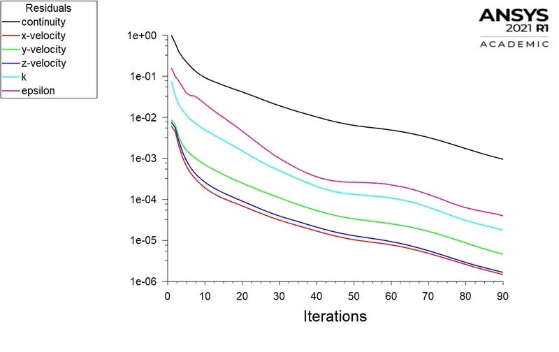
The residual plots are shown below. The solution attains a steady state in ~100 iterations. The same trend is followed in all cases.

2) Parameters Tab - Output Parameters:

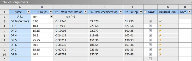
• Shown below is the final table of Design Points with all Input parameters and corresponding outputs.
• The MFR is negative in magnitude that indicates that the mass is moving out of the area.
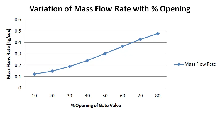
• The MFR increases gradually with an increase in the opening of the gate as expected.
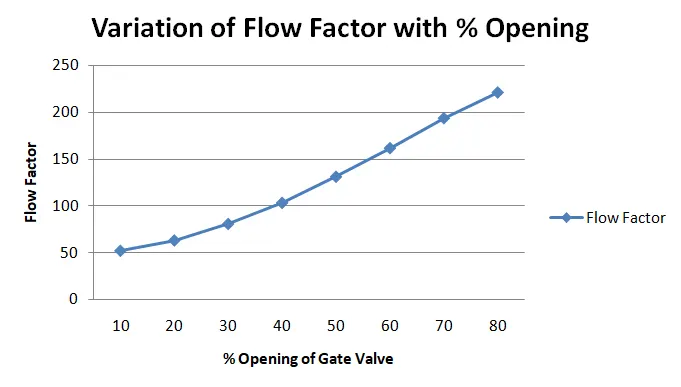
• The Flow factor and the Flow coefficient as well, increase gradually with an increase in the opening which is an expected result.
• The trends of MFR and Flow factor wrt % Opening is shown below. Line plot for Flow Coefficient is not plotted as it will be similar to the flow factor.

3) Velocity contours, Pressure Contours, and C/S View of Geometry for few cases:

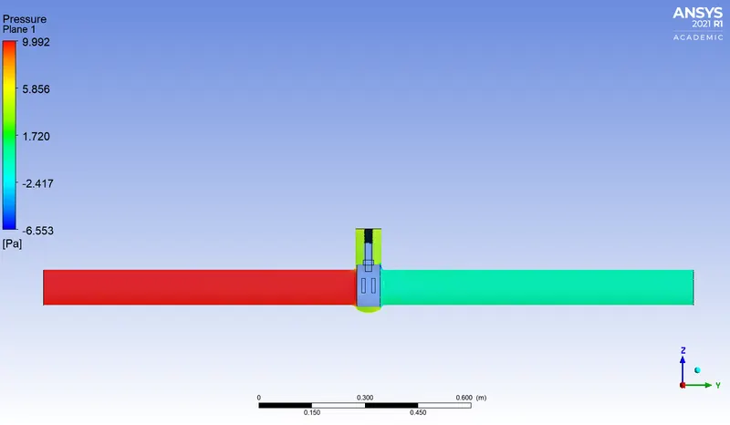
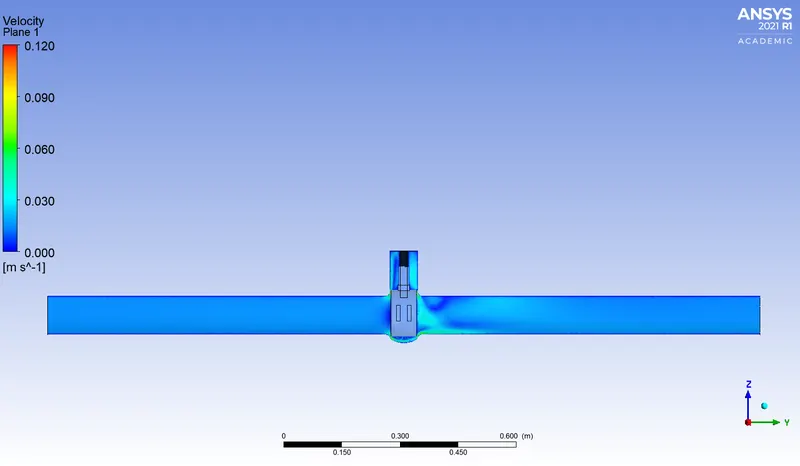
Design Point #0 - 5.05 mm Lift:

Design Point #5 - 25.25 mm Lift:

Design Point #8 - 40.4 mm Lift:

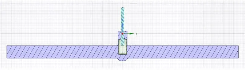
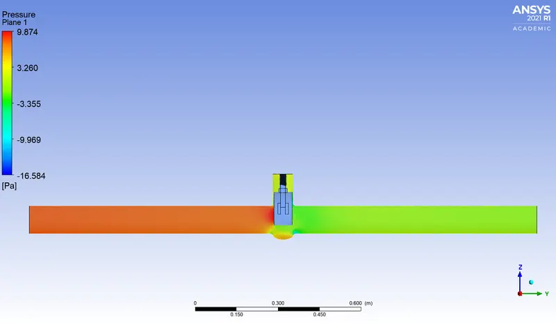
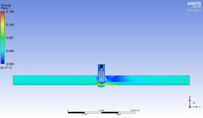
• The rise in the position of the Gate Disc can be observed from the C/S view of each case. The fluid volume gets updated automatically to the new position of the Gate Disc without user intervention.
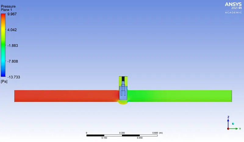
• The pressure contour shows a similar trend. The Inlet of the valve is pressurized due to the partial opening of the gate. Just after the gate, there is a region of negative gauge pressure followed by a gradual increase in the pressure up to 1 atm at the exit.
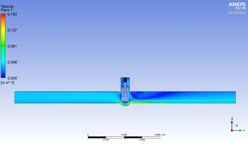
• The velocity remains a constant at the Inlet length up to the valve. The magnitude of water increases as the effective area of C/S for the water to flow decreases. Just after the gate valve, there exists a region where there is no water present in the fluid domain due to the blockage of water by the Gate. This explains the formation of the negative gauge pressure region.
• Water then attains a uniform magnitude across the cross-section of flow at the Outlet.
• Depending on the % opening of the Gate, the velocity magnitude, pressure magnitude change. The pressure drop is bigger when the gate % opening is less. The velocity at the outlet is higher when % opening is larger.

CONCLUSION:

A Parametric study is conducted on the Gate Valve by varying the % opening of the gate. Output parameters such as the Mass Flow Rate (MFR), the Flow coefficient, and the Flow factor is calculated in each case by specifying them as 'Output Parameters'. The trend of variation of MFR and Flow coefficient wrt the % Opening of Gate is plotted. The velocity contour and the pressure contours are observed.