Literature review on Introduction to Turbulence Modeling and RANS based turbulence models
AN INTRODUCTION TO TURBULENCE MODELING:
References:
- Fluid Mechanics Fundamentals and Applications by Yunus Çengel, John M. Cimbala
- https://www.fluidmechanics101.com/
Turbulence is characterized by high frequency and random fluctuations in the velocity flow field. The instantaneous velocity in a turbulent flow can be thought of as a sum of the following terms: A time-averaged flow velocity and fluctuating velocity.
u(x,y,z,t) = `bar u(x,y,z) + u'(x,y,z,t)`
Fluctuations are observed not only in velocity but in pressure and temperature as well. The magnitude of these fluctuations is not huge compared to the magnitude of the average velocity, but the frequency of the fluctuations (~1000 to 1500 per second) is what causes a drastic change in the behavior of the flow of fluid. This unique behavior can be attributed to swirling eddies present in the flow. These swirling eddies transport mass, momentum, and energy at a much faster rate than that of molecular diffusion in laminar flow. Hence, mixing is an inherent property of turbulent flow.
Solving the Navier-Stokes equation by substituting the expression for instantaneous velocity results in what is called the Direct Numerical Simulation (DNS). A DNS simulation, if performed, would yield the most accurate results but, for doing such a simulation, the cell/ mesh size needed is incredibly small. Abiding by the CFL criterion, the timestep for such a simulation will be small as well, which would make a DNS Simulation impractical for industrial usage. To overcome this problem, Turbulence Models are used. Turbulence models are used to capture the effects of turbulence up to a certain accepted accuracy and get away with larger grid size.
Turbulence Models are of two classes that shown below in increasing order of accuracy:
- Reynolds Averaged Navier Stokes (RANS)
- Large Eddy Simulation (LES)
Most of the engineering simulations are done using RANS as it requires less computation cost and time. LES is generally used as a research tool. This challenge focuses on the RANS Turbulence model only as LES is out of the scope of the course.
REYNOLDS AVERAGED NAVIER-STOKES (RANS) TURBULENCE MODEL:
RANS solves equations for the time-averaged velocity field. The approach used is the same as the textbook definition. The instantaneous velocity is considered as a sum of a time-averaged value and a fluctuating value. This is called Reynolds Decomposition.
Derivation:
Assume a flow v with a time scale T. Let `tunderset(i nt)()` denote a turbulent time scale that is much lesser than T.
The Reynolds decomposition is given by u(x,y,z,t) = `bar u(x,y,z) + u'(x,y,z,t)` (A)
The first term on the RHS is called Time Averaged quantity and the second one is called Fluctuating quantity. When the fluctuating term is time-averaged for enough duration, it amounts to 0. This is a result to be remembered.
`1/(tunderset(i nt)()) int_0^(tunderset(i nt)())u'(x,y,z,t) = 0`
Now the Continuity Equation is considered:
Applying the Reynolds decomposition on the Continuity equation and time averaging it, we get :
`1/(tunderset(i nt)()) int del/(delx)[baru + u']dt + 1/(tunderset(i nt)()) int del/(dely)[barv + v']dt = 0`
Integral over fluctuating term is 0, hence what remains is
`(delu)/(delx) int_0^(tunderset(i nt)()) dt/(tunderset(i nt)()) + (delv)/(dely) int_0^(tunderset(i nt)()) dt/(tunderset(i nt)()) = 0`
`implies frac{delbaru}{delx} + frac{del barv}{dely} = 0` (B)
Next, the Momentum Equation is considered:
Some simplification is needed to the Momentum equation before applying the Reynolds decomposition; The seconds order gradients in 'X' direction are neglected in the RHS of the equation as they are negligible in magnitude compared to the gradients in 'Y' direction.
`rho((delu)/(delt) + u(delu)/(delx) + v(delv)/(dely)) = -(dp)/dx + mu(del^2u)/(dely^2)`
Now introducing, X component of velocity multiplied by Continuity eqn at LHS,
`(delu)/(delt) + u(delu)/(delx) + v(delv)/(dely) + u((delu)/(delx) + (delv)/(dely)) = -(dp)/(rhodx) + nu(del^2u)/(dely^2)`
Combining like terms and using product rule formula `del/(dely)(uv) = u(delv)/(dely) + v(delu)/(dely)` to simplify, we get
`implies (delu)/(delt) + 2u(delu)/(delx) + del/(dely)(uv) = -(dp)/(rhodx) + nu(del^2u)/(dely^2)`
`implies (delu)/(delt) + (del)/(delx)(u^2) + del/(dely)(uv) = -(dp)/(rhodx) + nu(del^2u)/(dely^2)`
Now, the Reynolds decomposition can be applied to the momentum equation.
`implies int_0^(tunderset(i nt)())(del(baru + u'))/(delt) dt+ int_0^(tunderset(i nt)())(del)/(delx)(baru + u')^2 dt+ int_0^(tunderset(i nt)())del/(dely)((baru + u')(barv + v')) dt= -int_0^(tunderset(i nt)())(d(barp + p'))/(rhodx)dt + int_0^(tunderset(i nt)())nufrac{del^2(baru + u')}{(dely^2)}dt`
Expanding the above equation, the integral of fluctuating terms will become 0. Rearranging, we get:
`implies (delbaru)/(delt) + (del)/(delx)(baru^2) + del/(dely)(barubarv) = -(dbarp)/(rhodx) + nu(del^2baru)/(dely^2) -1/(tunderset(i nt)()) int_0^(tunderset(i nt)()) del/(delx)(u')^2dt -1/(tunderset(i nt)()) int_0^(tunderset(i nt)()) del/(dely)(u'v')dt` (C)
The equation obtained (C) looks similar to the original Momentum equation except that it is time-averaged and has two new terms on RHS. Let us call these two new terms (a) and (b)
An important assumption is made at this point in the derivation. We know that the thickness of the turbulent boundary layer is very small. Within this small thickness, the velocity of flow changes drastically along the 'Y' direction. Along the direction of flow, the velocity gradient that exists is negligible in magnitude compared to the velocity gradient in the 'Y' direction. Hence, the term with a gradient along the 'X' axis is neglected. Term (a) is neglected.
`implies (delbaru)/(delt) + (del)/(delx)(baru^2) + del/(dely)(barubarv) = -(dbarp)/(rhodx) + nu(del^2baru)/(dely^2) -1/(tunderset(i nt)()) int_0^(tunderset(i nt)()) del/(dely)(u'v')dt`
On re-arranging the RHS, we get the final expression.
`implies (delbaru)/(delt) + (del)/(delx)(baru^2) + del/(dely)(barubarv) = -(dbarp)/(rhodx) + 1/rho*del/(dely)[mu(del baru)/(dely) -rho/(tunderset(i nt)()) int_0^(tunderset(i nt)())(u'v')dt]` (D)
Inference:
The LHS of the final expression (D) represents the time-averaged inertial terms. The first term of the RHS is the time-averaged pressure gradient term and the second term represents the time-averaged momentum diffusion.
Consider the time-averaged Momentum diffusion term.
`1/rho*del/(dely)[mu(del baru)/(dely) -rho/(tunderset(i nt)()) int_0^(tunderset(i nt)())(u'v')dt]`
The expression is a sum of two terms. The first term `mu(del baru)/(dely)` is called the Molecular Viscosity and signifies that momentum is diffused due to molecular viscosity. The second term `rho/(tunderset(i nt)()) int_0^(tunderset(i nt)())(u'v')dt` signifies that momentum is diffused by turbulence. When the expression in the bracket in (D) is multiplied with the derivative outside the bracket in RHS, expressions for the Viscous Stress and the Reynolds Stress are obtained respectively.
About Reynolds Stresses:
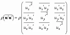
The complete Reynolds Tensor is shown. The Reynolds stresses represent the shear stress per unit area due to the eddy motion of fluid particles. It describes how the momentum gets diffused due to turbulent fluctuations. For example, Let a flow be considered primarily in 'X' direction; Now, if a small positive fluctuation along the 'Y' axis is introduced, (i.e. a fluid particle is injected along the Y-axis), this will cause a slow down in the velocity/momentum of particles along the 'X' axis. This is the essence of turbulent shear stress.
Hence, in the product, u'v', one term has a negative effect on the other. If u' increases `implies` v' decreases, and vice-versa. So, the Reynolds shear stress term is always written with a negative sign to make the overall product a positive quantity.
`tauunderset(turb)() = -rhobar(u') bar(v') = muunderset(t)()frac{delbar(u)}{dely}`
At this point, turbulence modeling would mean, accurately calculating the Reynolds Tensor Term. From the equation shown above, the turbulent viscosity (`mu underset(t)()` ) is directly related to the Reynolds stresses.
Today, sophisticated transport equations involving turbulent kinetic energy are solved to approximate `mu underset(t)()`. Upon finding `mu underset(t)()`, the Reynolds stresses can be obtained using the Boussinesq hypothesis. Upon obtaining the Reynolds stresses, the RANS system of equations can be closed.
Contrasting Molecular and Turbulent Viscosities:
The turbulent viscosity is also called Eddy Viscosity. The turbulent viscosity accounts for momentum transfer by Eddies. It is not a fluid property but, it depends on the conditions of flow. The eddy viscosity tends to 0 near the wall as the No-slip condition prevails at the wall. But inside its core region, the turbulent boundary layer, it can be several thousand times the value of molecular diffusivity in its core region. The earliest theory to estimate the turbulent viscosity was the Prandtl Mixing Theory in the 1900s which introduced the concept of 'Mixing Length (`lunderset(m)()`)' and stated that the average size of the eddies is primarily responsible for mixing.
On the other hand, Molecular Viscosity is the internal friction between layers of fluid caused due to the momentum exchange of the molecules. Unlike turbulent viscosity, molecular viscosity is a property of the fluid. Molecular viscosity is only dominant in its core area i.e. the Viscous sub-layer within the boundary layer.
UNDERSTANDING THE REGION OF DOMINANCE OF THE DIFFERENT VISCOSITIES:
The turbulent boundary layer is generally divided into 3 categories based on the dominant forces:
- Viscous Sub-Layer: Region inside Turbulent Boundary Layer where viscous stresses dominate over Reynolds stresses
- Buffer Layer: Region inside Turbulent Boundary Layer where Reynolds stresses become more significant but does not dominate
- Log-Law layer: Region inside Turbulent Boundary Layer where Reynolds stresses dominate over viscous stresses
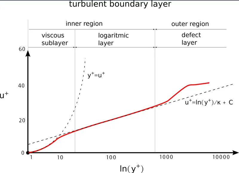
In turbulence modeling, it is important to know the operating region of the boundary layer. To find out the operating region, the flow field variables have to be converted to Near Wall Variables. For this purpose, two dimensionless quantities u+ and y+ are used.
A) The Near Wall Velocity `u+` is defined as `u+ = frac{bar(u)}{u overset(**)()` where `u overset(**)()` is called Friction Velocity and defined as `u overset(**)() = sqrt(frac{tau underset(s)()}{rho}`. U+ physically represents the ratio of time averaged velocity to the rate at which the turbulent boundary layer is growing.
B) The Non-Dimensional Wall Distance `y+` is defined as `y+ = frac{y}{L underset(char)()}` where the characteristic length `Lunderset(char)() = frac{u overset(**)()}{nu}` which has units of 'metres'. Y+ physically represents how thick the turbulent boundary layer is. Y+ values between 1 and 10 indicate that the operating region is the Viscous Sublayer and y+ values greater than 30 indicate that the operating region is the Log-Law region. On plotting U+ and Y+, the Law of the Wall is obtained.
It has been found that in the viscous sub-layer, the expression `u+ = y+` holds good and the expression `u+ = 1/kln y+ C` called the Log Law holds good in the Outer Region. k and C are experimental constants.
APPLICATION OF Y+:
Y+ tells the operating region of the turbulent boundary layer which primarily assists in determining the location where the first cell of the mesh is to be placed. This is of vital importance because different turbulence models are designed for different applications. For example, the RANS-based `k-omega` SST turbulence model is a low Reynolds number turbulence model. A low Reynolds number model would mean that it is primarily designed for the viscous sublayer. This in turn implies that the cells of the mesh must be refined to an extent where the first layer of cells must be within the thickness of the viscous sublayer to capture information accurately.
Similarly, the RANS-based standard `k-epsilon` class of turbulence models are high Reynolds number turbulence models. This means the cells of the mesh need not be much refined as much as in the previous case. Its first-layer of cells must lie just within the log law thickness with 30<Y+<100. There are also other turbulence models from the class of `k-omega` which uses automatic wall treatment that has an inbuilt blending function that helps the solver choose the equations to be solved based on values of Y+ between 30 and 300. Shown below are some commonly used RANS-based turbulence models and their applications.
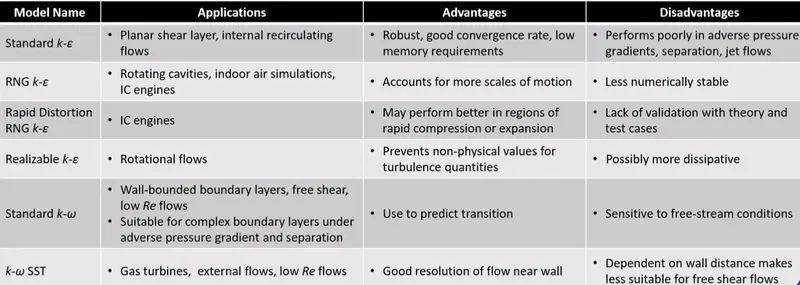
The turbulence model solves sophisticated transport equations involving turbulence kinetic energy to obtain the turbulent viscosity. Once the `mu underset(t)()` is obtained from the turbulence model, it is then applied to the Boussinesq hypothesis to obtain the Reynolds stresses. Upon obtaining the Reynolds stresses, the RANS system of equations is closed.