Simulating Flow over a Cylinder using Fluent

OBJECTIVE:

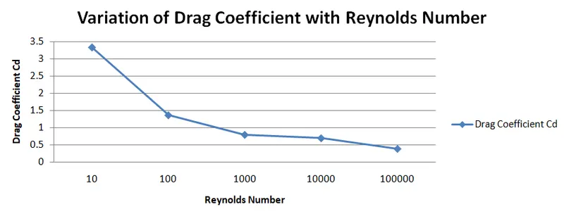
The challenge aims at conducting an external flow simulation over a cylinder. The Vortex Shedding phenomenon is to be captured and related parameters such as the Strouhal Number of the transient lift, the coefficient of Lift, and the coefficient of Drag are to be determined. The variation of coefficient of drag wrt Reynolds number is to be determined. The angle of separation is to be estimated using an approximate technique wrt different Reynolds number.

SOFTWARES USED:

1. Ansys Fluent 2021 R1

FLOW PAST A CIRCULAR CYLINDER AND VORTEX SHEDDING:

When a bluff body is placed in a free stream flow, separation of streamlines occurs and a wake region is formed. Depending on the shape of the bluff body and the Reynolds numbers [usually Laminar], there is an onset of instability in the wake and results in periodic shedding of vortices. This is called Vortex Shedding. Viscous effects and rotations are significant in the wake region.

The Vortices are formed are not simultaneous on both sides of the body but are rather staggered. A growing vortex is constantly affected by the formation of a new vortex which has a negative sense in rotation. This results in a cancellation effect of the growing vortex and it becomes weaker in strength. The vortex is then detached from the viscous layer and moves with the flow as a free vortex. This mechanism keeps repeating at a definite frequency and the phenomenon is known as vortex shedding. This propagation of alternating shed vortices in the wake of a blunt body is called Von Karmann Vortex Street.

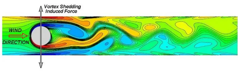
Depending on the Reynolds number, flow over the cylinder can be classified into different regimes as shown. In this challenge, a steady-state simulation and a transient simulation is performed for a Reynolds number of 100 i.e., in the Laminar regime. The steady-state study will be further extended to higher Reynolds numbers and its effect on the coefficient of drag is studied.

0 < Re < 4	Creeping Flow
4 < Re < 48	Laminar Flow with steady separation forming symmetric contra-rotating pair of vortices
48 < Re < 180	Laminar Flow with period Vortex Shedding
180 < Re < 400	Transition in Wake [TiW] Regime

Effect of vortices on Lift and Drag:

Vortices are high-speed rotational flows that have low pressure in the center. In a clockwise vortex (say), the upper side of the vortex has a local high velocity (since the velocity vector is along the flow direction), low-pressure region. The lower side of the vortex has low speed and is a local high-pressure region. This difference in pressure causes a lift. The higher the speed of rotation of the vortex, the more will be the lift. The vortex that is shed next will have a negative lift as the sense of rotation is opposite. Whenever the body experiences lift, it immediately experiences a reactive force in the opposite direction. Hence, in a vortex street, the body begins to oscillate in the transverse direction of the flow. If this frequency of oscillation is close to the natural frequency of the body, it may lead to resonance and structural damage!

The flow, when it comes in contact with the bluff body, has the maximum pressure [max stagnation pressure]. The pressure behind the body is much lower due to the formation of vortices that have low-pressure centers. This difference in the pressure increases the drag drastically. This drag is called Pressure drag.

Strouhal Number:

The Strouhal number represents the ratio of inertial forces due to the local acceleration of the flow to the inertial forces due to convective acceleration. Hence, in periodic motions, the Strouhal number is associated with the oscillations of the flow due to the inertial forces relative to the changes in velocity due to the convective acceleration of the flow field. It is given by `St = frac{fD}{Uunderset(oo)()}`,

where f is the frequency of formation of the vortices, D is the characteristic length of the bluff body, and `Uunderset(oo)()` is the freestream velocity. Each bluff body has a particular Strouhal number depending on its characteristic flow separation. A wider wake will result in a low Vortex shedding frequency.

High Strouhal numbers indicate that oscillations dominate in the flow whereas low Strouhal numbers indicate that oscillations are washed off quickly by the flow. Also, the spacing between vortices is dependant on the Strouhal number. In this challenge, the Strouhal number corresponding to the transient lift is calculated using Fast Fourier Transform (FTT).

CASE SETUP IN ANSYS FLUENT:

Firstly, flow over the cylinder is simulated as a steady-state stimulation for various Reynolds numbers of 10, 100, 1000, 10000, 100000. The coefficient of lift and drag is found. The variation of the drag coefficient wrt the Reynolds number is determined. The angle of separation is determined. Secondly, the case is simulated using the transient solver at Reynolds number of 100 and the Strouhal number is calculated.

A) GEOMETRY:

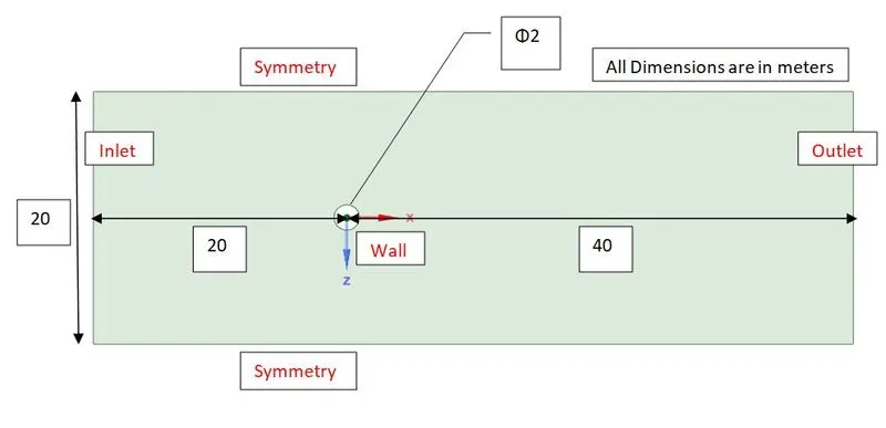
Shown below is the fluid domain. The simulation is a 2D simulation and the cylinder is represented by a 'Wall' boundary condition. The diameter of the cylinder is 2 meters. The upstream length of the cylinder is 10*D = 20 meters and the downstream length is 20*D = 40 meters. The top and the bottom is given 'symmetry' boundary condition.

B) MESHING:

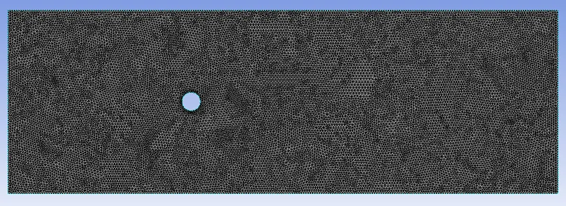
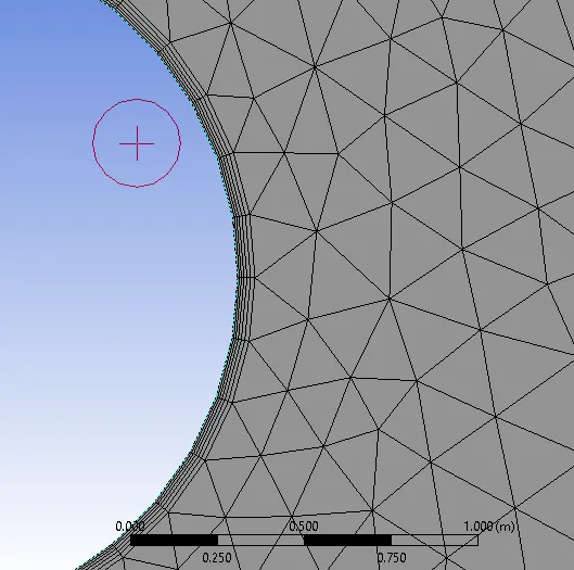
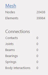
Ansys meshing provides a default mesh which is 'quad dominant' that is automatically generated when the module opens. Firstly, the mesh is changed to 'all triangles'. Secondly, the base mesh is set to 1 meter. Next, to ensure that the 2D cylinder retains its curvature, mesh 'edge sizing' is added with 36 divisions on the edge of the cylinder. To capture the physics around the flow, mesh inflation regions are added. A first layer thickness of 0.005 meters is given and the number of layers is set to 6 with a default growth rate of 1.2. With these settings, shown above is the mesh generated.

After a process of trial and error, the base mesh is changed to 0.25 meters.

C) SETTING UP CASE IN FLUENT:

• Firstly, a mesh check is performed in fluent.
• Next, a user-defined material is added to suit the requirements. Under the 'Physics' tab, the 'Materials' is selected, and the properties of 'air' are copied and renamed as user-defined material. The density is 1 and viscosity is specified as 0.02 so that the calculated Reynolds number is 100. The existing 'air' is removed from the cell zone.
• The solver type is set to pressure-based-steady. Next, according to the operating Reynolds number, in the 'Reference Values' tab, different parameters such as the dimensions, the velocity, and the boundary from which the normalized flow variables are to be calculated are specified.
• Depending on the operating Reynolds number, either the turbulence model is specified as 'laminar' or the model itself. To come up with the right turbulence model, the y+ is calculated. Shown below is the calculation of y+ for the Reynolds number of 10,000.

Re = 10000; `mu` = 0.02; `Uunderset(oo)()` = 100 m/s; (first layer height) = 0.005 m, `rho` = 1.

`y+ = frac{yoverset(star)()*u}{nu}` --------------------------------------------------------(A)

`u = sqrt(frac{tauunderset(w)()}{rho})` ----------------------------------------------------(B)

`tauunderset(w)() = 0.5 rho Cunderset(f)() Uunderset(oo)()^2` --------------------------(C)

`Cunderset(f)() = 0.0576 *Re^(-1/5)` -------------------------------------------------------(D)

Re = 10000 `implies` `Cunderset(f)()` = 0.009128984 `implies tauunderset(w)()` = 45.64492 N/m^2 `implies` u = 6.756102 m/s.

Substituting the above values in equation A, we get y+ = 1.689 `implies` the `k-omega` SST turbulence model is chosen for this case.

• Next, the boundary conditions are specified as per the Reynolds number. The freestream velocity of the flow at the inlet is changed as per the Reynolds number keeping the density and viscosity constant. The pressure at the outlet is 1 atm.
• Under the 'Solutions' tab, the solution methods are specified. The SIMPLE scheme is chosen to solve the problem. Next, to observe the vortex shedding, a monitor point is created in the geometry at 10 meters downstream to the cylinder center.
• Monitor plots such as the 'vertex averaged velocity magnitude' at the monitor point, coefficient of lift, and coefficient of drag on the cylinder surface (wall) are specified.
• In addition, the velocity and pressure contours are set up. Lastly, to estimate the separation angle, a wall shear stress plot is set up with the XY Plots option under the 'Results' tab.
• Finally, the convergence tolerance criteria are unchecked for the residuals as it is required to run the case till the user-specified iterations/timesteps.
• The solution is then initialized using 'Hybrid Solver' and then run for 350-450 iterations depending on convergence.
• The transient case uses the same settings and specifications except for the solver type, which is set to transient and the simulation end time is set to 0.5 seconds with iterations of 500. This would imply that the flow time of the simulation is 500 X 0.5 = 250 seconds.

RESULTS:

A) CONVERGENCE PLOTS (STEADY AND TRANSIENT):

a) Steady:

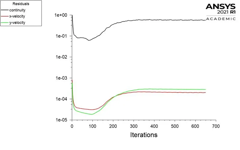
• The main objective of the challenge is to capture the vortex shedding phenomenon. It is of essence to capture the physics with a trade-off in the accuracy. Hence, the convergence tolerance criteria are disabled. From the plot below, it can be said that the case has achieved convergence and the resides are accurate to one decimal place.

b) Transient:

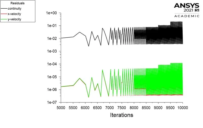
• A repeating pattern with an increase in the magnitude of residues is obtained. This implies that the transient case has converged. By disabling the convergence tolerance criteria, a tradeoff between the physics of the problem and the accuracy is made.

B) COEFFICIENT OF LIFT, DRAG, AND SEPARATION ANGLE WRT REYNOLDS NUMBER:

a) Coefficient of Lift:

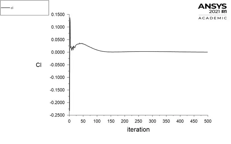
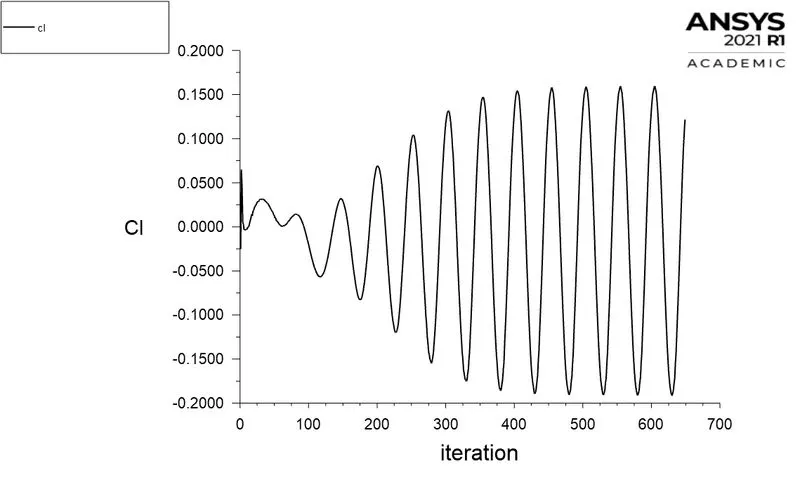
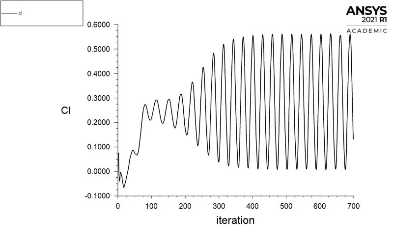
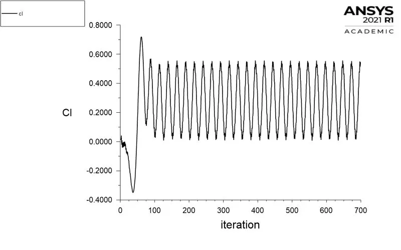
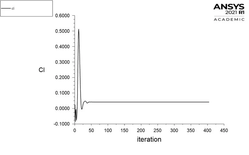
Using 'Report Definition'==> 'Force Reports' ==> 'Lift', the plot of coefficient of lift on the wall (cylinder) wrt iterations can be obtained. Shown below are plots of coefficient of lifts for Reynolds numbers 10, 100, 1000, 10000, 100000 respectively.

b) Coefficient of Drag:

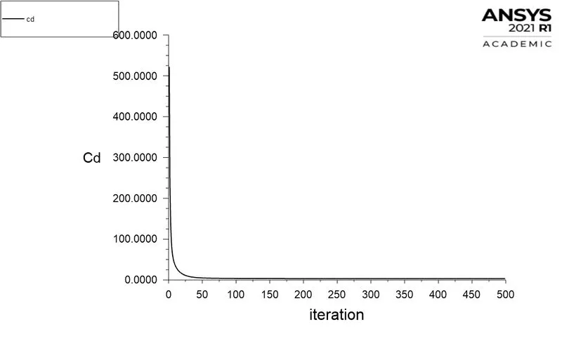
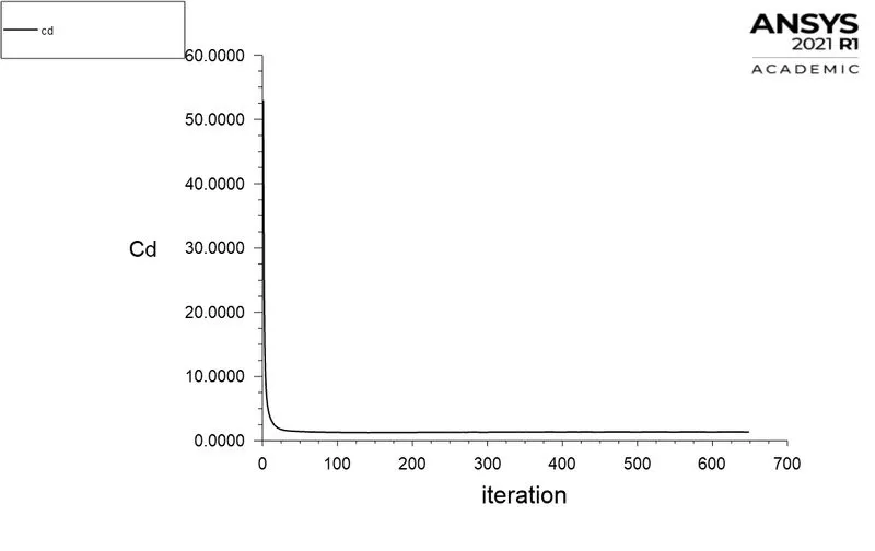
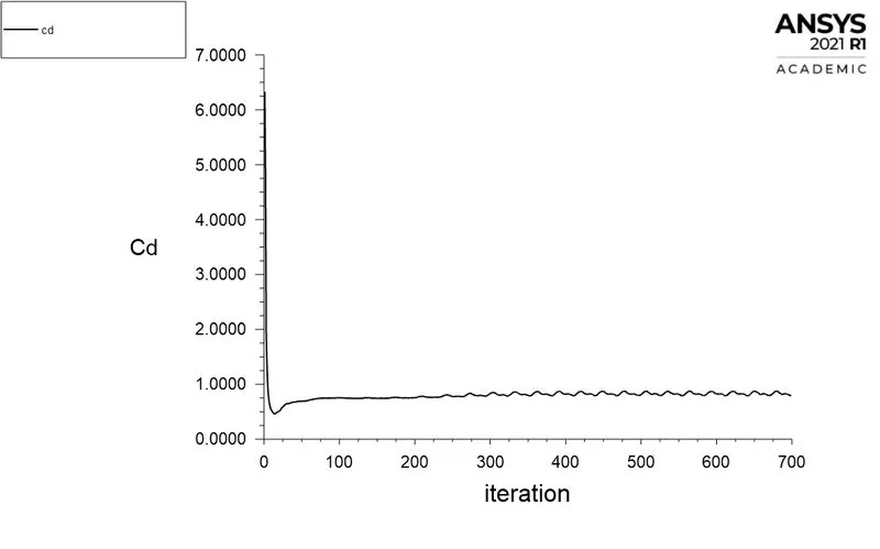
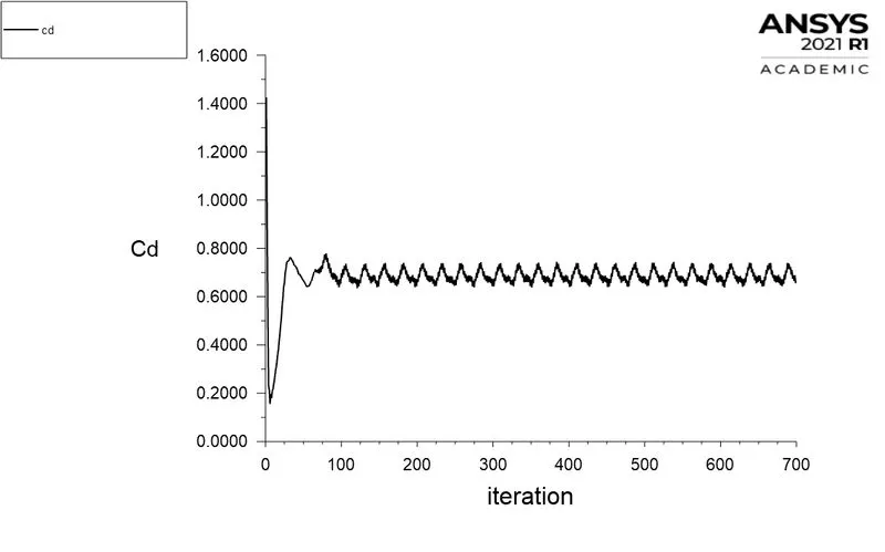
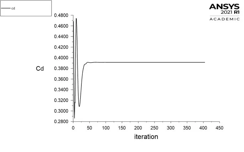
Using 'Report Definition'==> 'Force Reports' ==> 'Drag', the plot of coefficient of drag on the wall (cylinder) wrt iterations can be obtained. Shown below are plots of coefficient of drag for Reynolds numbers 10, 100, 1000, 10000, 100000 respectively.

c) Estimation of Separation Angle:

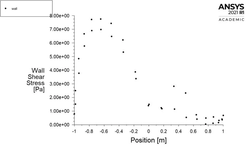
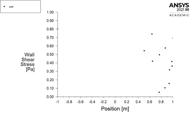
Flow separates under an adverse pressure gradient and at the point of separation, the wall shear stress is zero. The wall shear stress is plotted on the wall (cylinder) using the XY plot option under the 'results' tab. For demonstration, the estimation of the wall shear stress for the Reynolds number of 1000 is shown. Firstly, the wall shear stress on the cylinder is plotted. The plot on the right is the zoomed view of the plot on the left. The point of ~0 wall shear stress is eyeballed and this position is noted. Here it is close to 0.75 m from the origin (0 m).

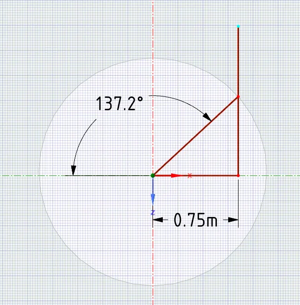
Next, SpaceClaim is opened and the following geometry is constructed as shown the angle of separation is calculated. The angle of separation is approximately calculated as 137.2 degrees for a Reynolds number of 1000.

d) Summarised Results:

Summarised below are different settings and steady-state values of the Separation Angle, coefficient of lift, and drag for various Reynolds Numbers.

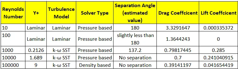
• The separation angle is almost 180 for Reynolds number 10. This is because, at this Reynolds number, it is creeping flow, and the fluid moves at slow speeds along with the geometry. At Reynolds number of 100, the separation angle is close to 180 as the velocity, in this case, is 1m/s which is not a high value. Since the technique involved in finding the angle of separation is not accurate, it is said that the separation angle is close to 180 as the zero value of shear is close to 1m from the origin. At higher values of Reynolds number, separation does not occur as the flow behavior is almost inviscid.
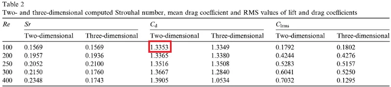
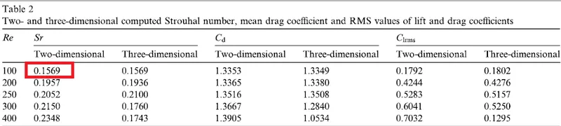
• The drag coefficient obtained for Reynolds number 100 is validated from [1] with an error of 2.17%. A plot of the variation of the Drag coefficient (Cd) wrt the Reynolds is shown below.

• The lift coefficient must be zero ideally in all cases of Reynolds number because the angle of attack of the cylinder is zero. But due to numerical diffusion, non-zero values that are close to zero are obtained.

C) VELOCITY AND PRESSURE CONTOURS WRT REYNOLDS NUMBER:

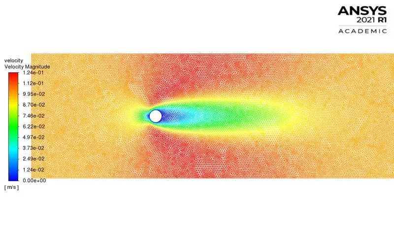
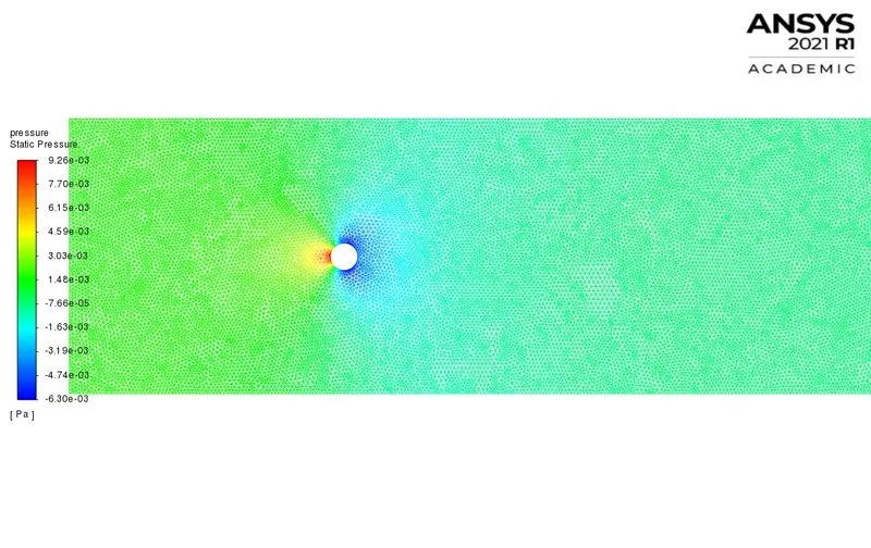
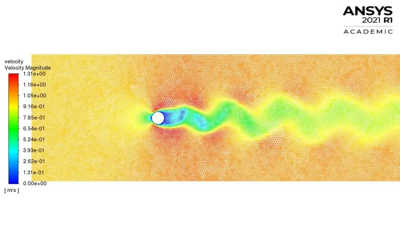
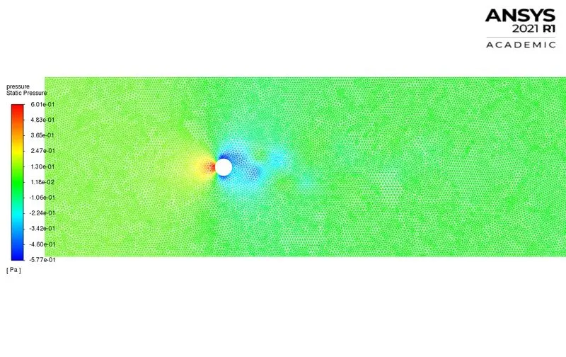
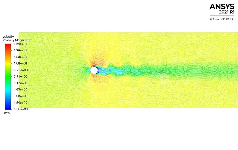
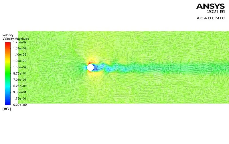
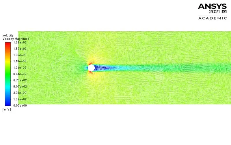
Shown below are contours of Velocity and Pressure for Reynolds numbers 10, 100, 1000, 10000, 100000 respectively.

a) Re = 10:

b) Re = 100:

c) Re = 1000:

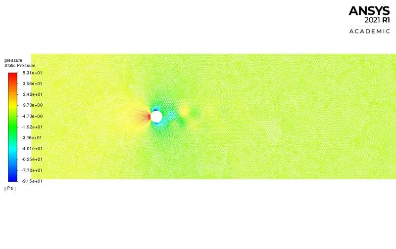
d) Re = 10000:

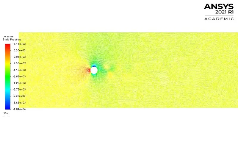
e) Re = 100000:

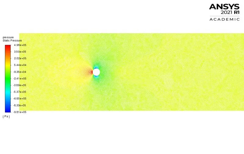
• The velocity contours show the behavior of flow with increasing Reynolds number. At Reynolds number of 10, it is the creeping flow regime and the flow does not separate.
• At Reynolds number of 100, Vortices are shed and a Von Karmann Vortex street is observed. Vortex Shedding occurs due to the interaction of the separated viscous layers of flow and is inherently a 3D phenomenon in nature.
• Beyond a Reynolds number of 350, turbulence effects become significant and the wake consists of eddies and vortices. The instability in the wake also becomes more significant in the third dimension. This is the beginning of the Transition in Wake [TiW] regime and the 2D contours of the wake do not capture the eddies and vortices accurately beyond this point.
• At very high values of Reynolds number, the flow starts to behave in an inviscid manner. Hence flow does not separate and vortices are not shed.

D) VELOCITY AT THE MONITOR POINT AND ANIMATION OF VON KARMANN VORTEX STREET AT REYNOLDS NUMBER 100.

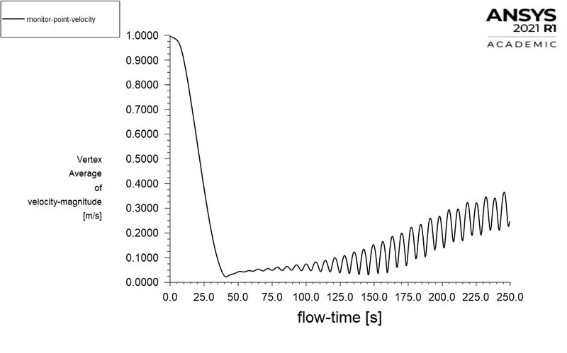
The magnitude of velocity is shown at the monitor point. This is a typical plot of the velocity magnitude which oscillates when vortices are shed. It can be observed that these oscillations occur at regular intervals and has a definite frequency.

E) CALCULATION OF THE STROUHAL NUMBER AT REYNOLDS NUMBER 100.

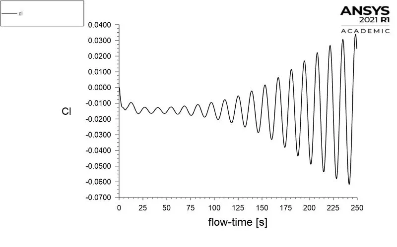
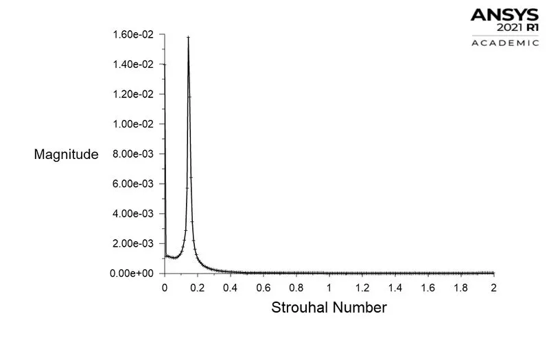
The Strouhal number of the transient lift is basically the nondimensional form of the frequency of lift. To calculate the Strouhal number corresponding to the transient lift, a Fast Fourier Transform (FTT) is performed on the converged lift data. The FTT converts signals from the time/space domain to a frequency domain. The Strouhal number is the value corresponding to the maximum magnitude of the amplitude in the obtained FTT plot. It is found to be equal to 1.4371258e-01 i.e., 0.1437. There is an error of 8.41% when compared with the results from [1].

CONCLUSION:

Steady simulations are performed at various Reynolds numbers and the effect on the coefficient of lift, coefficient of drag, and the separation angle is determined. Contours of velocity and pressure are plotted for various Reynolds numbers. The Von Karmann Vortex street is captured at a Reynolds number of 100. A transient simulation is performed at a Reynolds number of 100 from which the Strouhal number is estimated and validated with [1].

References:

[1]: Numerical Simulation of laminar flow past a circular cylinder; B.N. Rajani, A. Kandasamy, Sekhar Majumdar

[2]: Strouhal Number - Science Direct