2D Cavitation simulation using Converge

OBJECTIVE:

In this challenge, the phenomenon of Cavitation is simulated and studied in a diesel injector nozzle. A plot of the pressure difference across the nozzle vs cavitation zone length is drawn. The effect of the Cavitation on the mass flow rate supplied by the nozzle is studied.

SOFTWARES USED:

1. Converge Studio v3.0
2. Windows CMD and CYGWIN
3. Paraview

CAVITATION AND ITS EFFECTS:

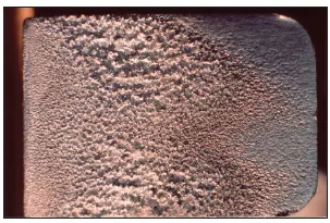
Let us say there is a liquid in a container. For the liquid to remain as it is, i.e., in a 'liquid state' at equilibrium with surroundings, the vapor of the liquid (present above the liquid) must exert a pressure equal to the saturation pressure of the liquid. (Saturation pressure is the critical pressure at which phase change takes place). If there is a difference in pressure, Evaporation takes place until there exists no pressure difference. In a phase change process, the vapor pressure and the saturation pressure are equal (measured close to the liquid-vapor interface). It is to be noted that vapor pressure increases with an increase in temperature. So, a substance can boil even at low temperatures given, its pressure is low.

The same phenomenon can take place in liquid flow systems such as turbomachinery, fuel injectors in engines, etc. At regions of low pressure, lets's say a sudden contraction in a duct or at the suction side of a pump system or at tips of impeller blades, at a fixed temperature of the liquid, if the pressure of the liquid falls below its vapor pressure, it results in vapourization. When the liquid vapourises, they form 'cavities of vapor' in the liquid continuum and flow with the liquid. When these bubbles enter a high-pressure region, they burst and cause pressure waves onto the solid surface which, over time, may damage/corrode the solid structure. This formation of bubbles at pressures lower than vapor pressure is called Cavitation. Cavitation results in erosion of the solid material generate vibrations and noise. Cavitation affects the performance of the fluid system and is an important aspect in designing fluid systems. Shown above is an image of the effect of corrosion on an aluminum surface.

In this challenge, Cavitation and its effects are simulated in a diesel fuel injector.

CAVITATION MODELLING:

References:

[1] 'Exploration of cavitation-induced erosion metrics in throttle flow simulations' by Argonne National Laboratory, Argonne, IL, USA and

[2] Fluid Mechanics Fundamentals and Applications by Yunus Çengel, John M. Cimbala.

Cavitation is studied using the 'Volume of Fluid' approach which is a subset of Multiphase flows. The geometry used is Winklhofer Throttle's “U” geometry for various pressure drops ranging between 20 to 100 bar. The Volume of Fluid (VOF) modeling section is activated automatically when a gas-liquid simulation is specified in Converge. The modeling approach used is that of [1], which is now described.

Diesel fuel is represented using tetradecane and trace amounts of `Nunderset(2)()` with a mass fraction of 5e-6. Both the liquid and gas phases are treated as incompressible. Cavitation and condensation are represented by a homogeneous relaxation model (HRM).

`frac{Dx}(Dt} = frac{barx-x}{theta}` where 'x' represents mass fraction of of vapour and `'theta'` is a relaxation timescale.

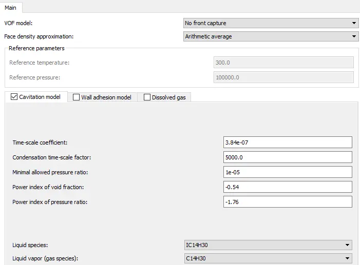
In this simulation, cavitation and condensation are assumed to occur at equal timescales. `'theta'` is represented by `theta = thetaunderset(o)() alpha^-0.54 psi^1.76` where `alpha` is the void fraction (fraction of gas phase and the liquid phase) and `psi` is the non-dimensional pressure ratio `frac{punderset(sat)()-p}{punderset(crit)()-punderset(sat)()}` and `thetaunderset(o)()` is a coefficient set to 3.84e-7.

CASE SETUP IN CONVERGE STUDIO:

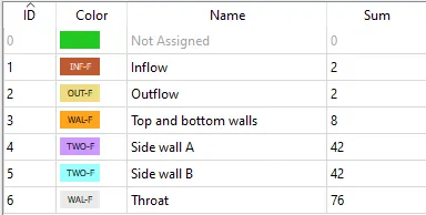
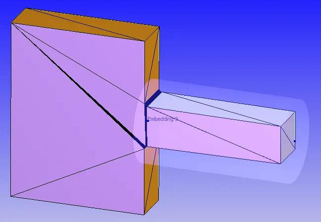
1) Geometry and flagging:

The geometry that is used to model a typical diesel injector is the Winklhofer Geometry. The bounding box of the geometry is of dimensions: 0.00202 X 0.0013125 X 0.0003 m which is comparable to a real time nozzle of a diesel injector.

2) Material:

Liquid Phase: IC14H30

Gas-Phase: C14H30

3) Mesh:

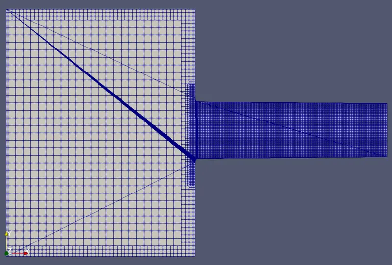
The base mesh used is 4e-5 m in all three directions. Cavitation happens close to the surface where a low-pressure region is formed due to sudden contraction. Hence in this example, cavitation can be assumed as a surface phenomenon. Hence, a fixed embedding is applied on the throat, the top and bottom walls, and in a cylindrical region around the throat. In addition, a fine refinement is needed in the 'throat' section of the nozzle to capture the smallest mass fractions of the gas phase tetradecane.

A velocity AMR and a species AMR on C14H30 are applied to the throat. All refinements are of scale 3 and 1-layered except that of top and bottom walls which is of the scale of 1.

4) Boundary Conditions:

Inlet: IC14H30 at a temperature of 300K. The inlet pressure is varied according to the given pressure difference array [30, 70, 100] bar. Hence the inlet pressures are 50 bar, 90 bar and 120 bar for a fixed outflow pressure of 20 bar.

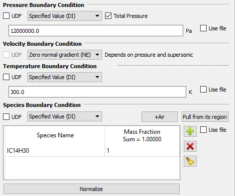
Outlet: The pressure at the outlet is fixed at a value of 20 bar. In the case of backflow, the backflow species is IC14H30 at 300K.

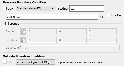
Top and Bottom Walls and throat: The Top and Bottom Walls and the throat are specified as a wall with the Law of Wall boundary condition at a temperature of 300K.

Side Walls: Sidewalls are given two_D boundary conditions.

5) Initial Conditions:

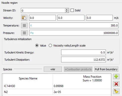
IC14H30 with a mass fraction of 0.99998 and N2 with a mass fraction of 2e-5 as mentioned above. The temperature of the region is 300K at a pressure of 100 bar.

6) Simulation and Time parameters:

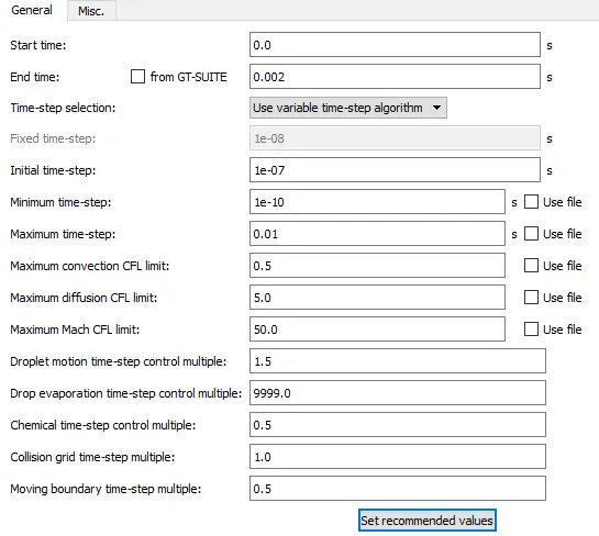
A full hydrodynamic simulation is performed with a transient solver. The N-S solver is set to PISO (Pressure Implicit with Splitting of Operators) which is predominantly used to handle unsteady simulations. It uses the concept of pressure correction; The algorithm uses 1 predictor step and 2 corrector steps to arrive at an accurate value for the pressure correction term. A density-based solver is chosen to deal with high-speed flows.

The end time of the simulation is considered as 0.002 sec which is a typical value for diesel injection. The max convection CFL limit is set to 0.5. which means that the velocity of the travel of information cannot travel more than half of a computational cell within one timestep. This will limit the simulation because the pressure difference across the nozzle is huge and high-speed flow will be generated across the nozzle in reality. But, a restriction is applied to the velocity of information computationally.

7) Volume of Fluid Setup (VOF):

The VOF model used is according to [1] which is described above. The liquid (IC14H30) and the gas species (C14H30) are explicitly mentioned.

8) Turbulence properties:

RNG `k-epsilon` turbulence model is set for the case. Generally, the standard `k-omega` SST model is suitable for capturing pressure drop. If details such as drag on impeller blades are to be captured, the `k-omega` SST turbulence model would be more suitable.

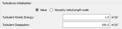
The (Initial Conditions) initial value of Turbulent Kinetic energy 'a' is assigned to the default value of 1 `m^2s^-2` and Turbulence Dissipation rate '`epsilon`' is assigned to the default value of 100 `m^2s^-3`.

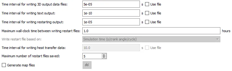
9) Output/ Post processsing variables reqd:

EXPORT OF INPUT FILES:

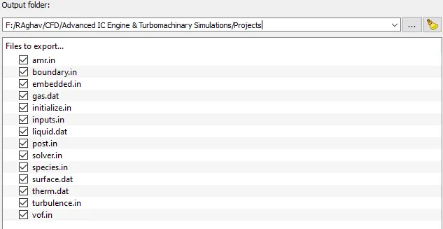
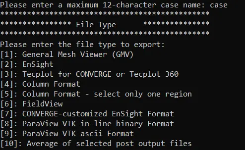
In Converge Studio, the case set-up of the problem is done. This essentially creates all the necessary input files for the Converge solver. Once the case setup is done, the input files are exported to a new folder. Shown below is the list of input files that have been generated by Converge Studio.

RUNNING THE SIMULATION:

A Command-line editor tool like Windows CMD or CYGWIN is used to set up the run. Here Windows CMD is used. Firstly, the location of the input files is navigated to and the Converge solver is called using the Command Line tool. For faster computational speed, parallel processing is set up on multiple cores using INTEL MPI software.

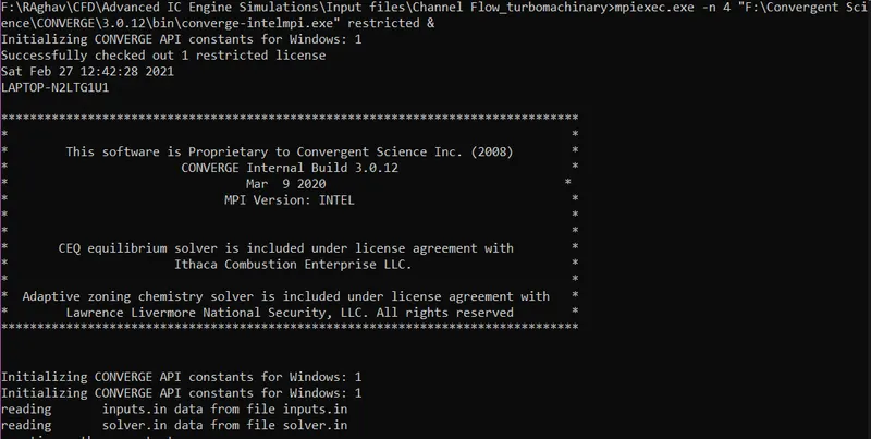
At the end of the run, the solver generates "post.h5" files (3D Output files) and ".OUT files" (Data files). The ".OUT" files contain data at mesh points. The 3D Output files are further post-processed using Converge post-processing tool into "Paraview VTK-Inline Binary format" to further analyze the case in Paraview.

RESULTS:

1) Mesh:

2) Void Fraction, Mass Fraction, Velocity Contour, and Cavitation Zone:

A) Pressure difference of 30 bar:

B) Pressure difference of 70 bar:

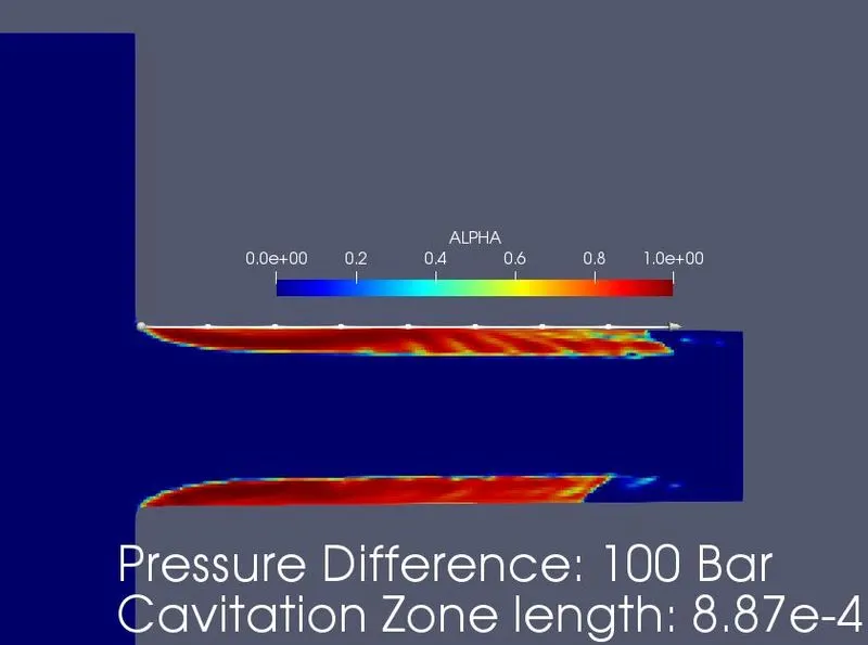
C) Pressure difference of 100 bar:

Inferences from the above Contours:

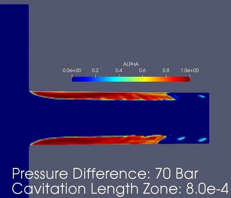
• From the velocity contours, it can be seen that at the regions close to the walls of the throat, there exists a low value of the velocity of flow. This region is occupied by the gaseous phase C14H30 which is observed from the void fraction (`alpha`) contour. A high value of `alpha` means the domination of the gaseous phase. This is the phenomenon of Cavitation.
• When the flow encounters a sudden contraction, recirculation zones of low pressure are formed just in the smaller area near the walls. If the pressure becomes low enough i.e below the saturation pressure of the liquid at the given temperature, the liquid is subjected to cavitation.
• The same inference can be proclaimed from the mass fraction contours. The mass fraction of liquid IC14H30 is high at all regions except the low-velocity regions i.e., near the walls of the throat where the mass fraction of gaseous C14H30 dominates.
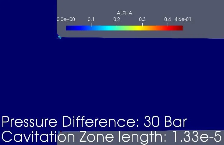
• The length of the cavitation zone is measured for different pressure differences in the void fraction plot using the line command in ParaView and is reported in meters (m) in the images above.
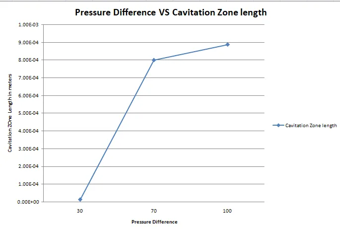
• For a pressure difference of 30 bar, there is hardly any cavitation zone. But as the pressure difference increases, the length of the cavitation zone increases drastically. This is because as the pressure difference increases, the velocity of the flow increases which results in an extended recirculation zone which in turn causes a larger cavitation zone. This is represented by the plot of Pressure Difference VS the Length of Cavitation Zone shown below.

2) Effect of cavitation on the Mass Flow rate:

Mass flow rate is a derived quantity. The contour of mass flow rate is obtained by multiplying the density and velocity of cell data in ParaView using the 'Calculator command'. After obtaining the MFR contour, the 'Plot over Line' command is used to make a line probe at the outlet of the nozzle. The MFR is measured normal to the outflow and along with the probe and the values are plotted along with the contours as shown.

A) Pressure difference of 30 bar:

B) Pressure difference of 70 bar:

C) Pressure difference of 100 bar:

Inferences from the above Contours and Plots:

• It is to be noted that the flow in the fuel injector is very high and for such high-speed flows, the no-slip condition hardly creates much resistance to the flow near the walls.
• Yet we observe that the mass flow rate is relatively less close to the walls of the throat compared to the throat's center and we get a distorted shape of the mass flow rate profile along the probe.
• This can be attributed to cavitation. It is because of cavitation that some of the liquid molecules are converted to gaseous phase that not only corrode the solid surface but also decrease the mass flow of the liquid exiting the control volume in a stipulated time thereby decreasing the performance of the fluid system.
• From the plots obtained from line probes, it is observed that huge fluctuations and distortions are seen in the mass flow across the outflow. These fluctuations become more violent with the increase in pressure difference. So, cavitation not only decreases the MFR, but the mass flowing out of the fluid system becomes unpredictable. This may pose a huge problem in cases like fuel injectors where accurate amounts of fuel are required for optimal combustion.

CONCLUSION:

1. Three cases were set up and run for Cavitation on Winklhofer Nozzle.
2. Plots for Velocity, Mass fraction, Void fraction were Post-processed in Paraview
3. A plot for the Pressure difference Vs Cavitation zone length was generated in excel.
4. The effect of Cavitation on the mass flow rate was studied.