CHT Analysis on Exhaust port

OBJECTIVE:

The aim of this challenge is to simulate Heat Transfer in an Exhaust Port using Ansys Fluent. The obtained Wall Heat Transfer Coefficient is compared with analytical relations. Temperature distribution contours are obtained.

CONJUGATE HEAT TRANSFER [CHT]:

Modes of Heat Transfer:

i) Conduction: Conduction is the mode of heat transfer that occurs from a more energetic particle to the adjacent less energetic particle and it takes place in a stationary medium. It is the most predominant mode of heat transfer in solids. It can occur in liquids and gases as well but with relatively diminishing efficiencies. In solids, conduction takes place through the movement of free electrons and Lattice vibrations.

ii) Convection: Convection is the mode of heat transfer between a solid surface and the adjacent fluid that is in motion. It involves the combined effects of conduction and fluid motion. Convection may be Free convection, Forced convection and it may occur with phase change like Boiling and Condensation. The aim of the convection study is to calculate the Heat transfer coefficient (HTC).

iii) Radiation: Radiation is the mode of heat transfer that takes place through Electromagnetic Waves [EM Waves]. This mode of heat transfer is the fastest and it does not require any medium for the propagation. Usually, at low temperatures [room temperatures], Conduction and Convection dominate over Radiation and hence effects of radiation would be neglected.

Conjugate Heat Transfer:

Conjugate Heat Transfer (CHT) is a class of simulation that is used to model heat transfer which occurs simultaneously within and between solid and fluid regions. The exchange of thermal energy takes place at the solid-fluid interface. The predominant mode of heat transfer in fluids is convection and in that of solids is conduction. CHT is performed when the user is interested in capturing the temperature distribution from the solid to liquid region. Examples include simulation of heat transfer in the Engine from the Engine block to the flowing coolant, etc. Different governing equations are solved in the solid domain and the liquid domain simultaneously and the temperature is estimated at the interface.

Equations solved in the solid domain:

Steady state heat conduction equation:

`Cunderset(p)()*rho(delT)/(delt) = nabla(knablaT) + Sunderset(h)()`

Equations solved in the fluid domain:

Navier Stokes Equations:

CASE SETUP IN ANSYS FLUENT:

I) Introduction:

The physical model of the problem is as follows: An exhaust manifold with 4 inlets and 1 outlet is present. Hot air at 700 K enters the manifold at 5 m/s in all four inlets. The hot air transfers energy to the inner solid wall by forced convection. The solid wall of the manifold is made of aluminum. Conduction is neglected. The outer wall convective Heat transfer coefficient (HTC) is given as 20 `W/(m^2K)`. The objective of the challenge is to estimate the inner wall HTC and obtain the temperature distribution on the outer solid wall.

II) Geometry:

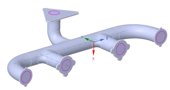
The geometry made up the geometry of the exhaust port in Spaceclaim is shown below. It consists of the outer solid region and inner fluid region [extracted using Volume extract] under one component. The 'share' option is enabled under the 'Workbench' tab in Spaceclaim to ensure the generation of conformal mesh. The interfaces of the solid and fluid regions that are shared are highlighted in 'pink' color.

III) Meshing and Y+:

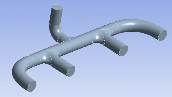
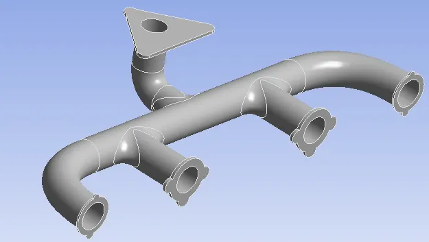
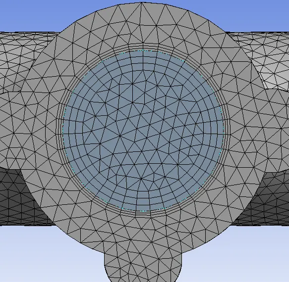
The fluid domain is shown on the left and the solid domain is shown on the right. It is pre-decided that the Standard `k-epsilon` turbulence model is to be used as capturing the boundary layer effects is not of interest. The range of Y+ in the standard `k-epsilon` turbulence model is 30 to 300. To obtain a base mesh a Y+ of 60 is chosen.

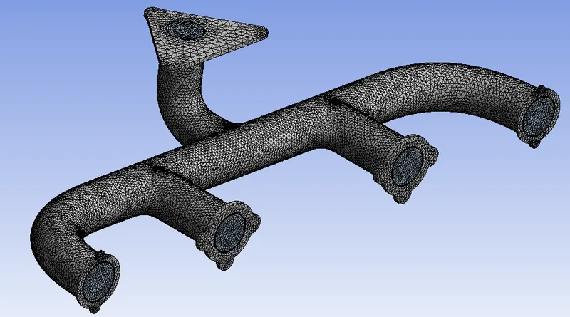
A basic mesh is generated without any specifications to take a look at the mesh and the total cell count is noted. As the cell count is not near the max cell limit, the mesh is refined. The maximum cell limit in the academic license is 512000 cells. Next, named selections are created- Inlet, Outlet, Solid_wall_convection, Inflation fluid layer. A Mesh body sizing with an element size of 15mm is to be added to the solid wall. Inflation layers are added to the fluid domain (named selection Inflation fluid layer). Inflation layer calculations were made from a standard inflation layer calculator available at www.fluidmechanics101.com

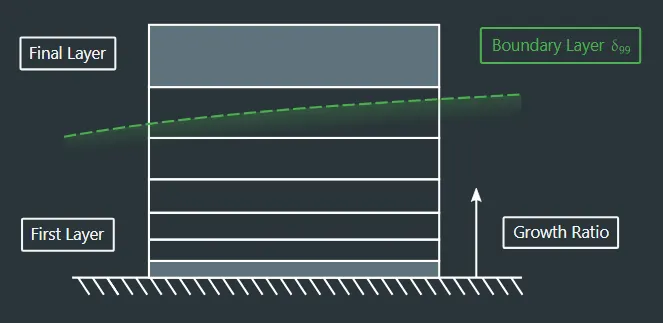
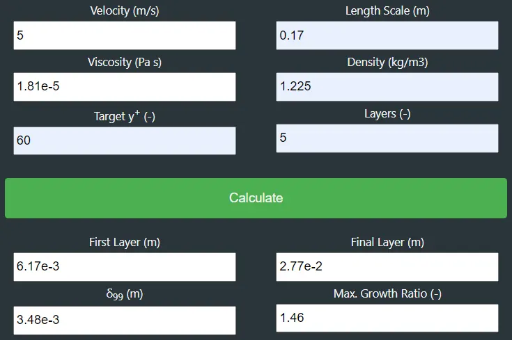
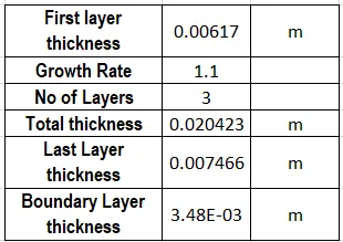
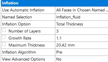
The first layer thickness is calculated as 0.00617 m based on a Y+ of 60. The total thickness for 3 inflation layers is calculated based on the formula of the sum of n terms of a GP as 0.020423 m. This is much bigger than the boundary layer thickness and holds with the decision that boundary layer effects are of no interest in this problem. The number of cells obtained in this refined mesh is 410137. This is the final mesh used in the problem.

IV) Fluent:

• A pressure-based, steady-state solver is used.
• Reference values are set as per the boundary conditions mentioned above to calculate the Wall Nusselt number for comparison.
• The energy equation is switched on.
• The Standard `k-epsilon` turbulence model is selected
• The solid material is chosen as aluminum and the fluid material is air. Material Properties are constant and do not vary.
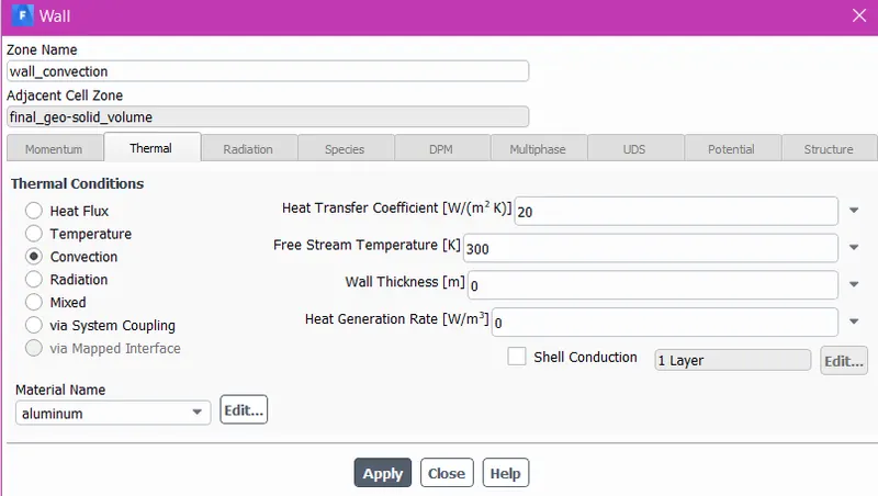
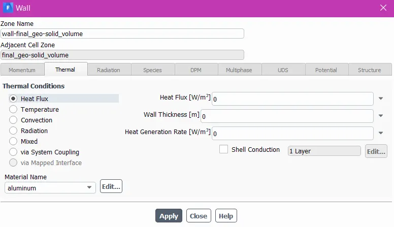
• Boundary conditions are specified. Velocity at all inlet named faces is 5 m/s. Pressure at the outlet is 1 atm. Outer Walls of the manifold are specified with 'convection' boundary condition and the HTC is set to 20 `W/(m^2K)`. Other walls that are not involved in heat transfer are set as an adiabatic boundary condition. This is done by specifying 0 heat flux.

• The solution scheme is a 'coupled' pressure velocity scheme.
• The solution is initialized using the Hybrid solver.
• Temperature contours, HTC Contour, the Y+ plot, and animation of the temperature contour are all set up under the 'results' tab.
• The time scale is set to 1 and the number of iterations is set to 500. The case is run.

RESULTS:

I) Convergence:

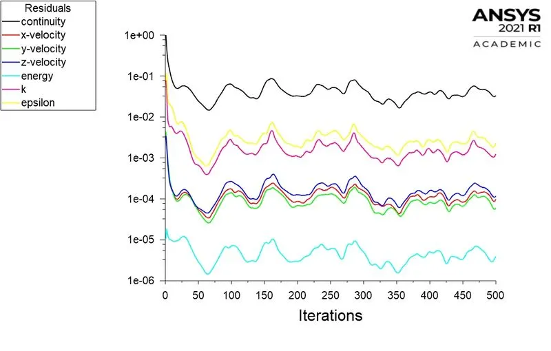
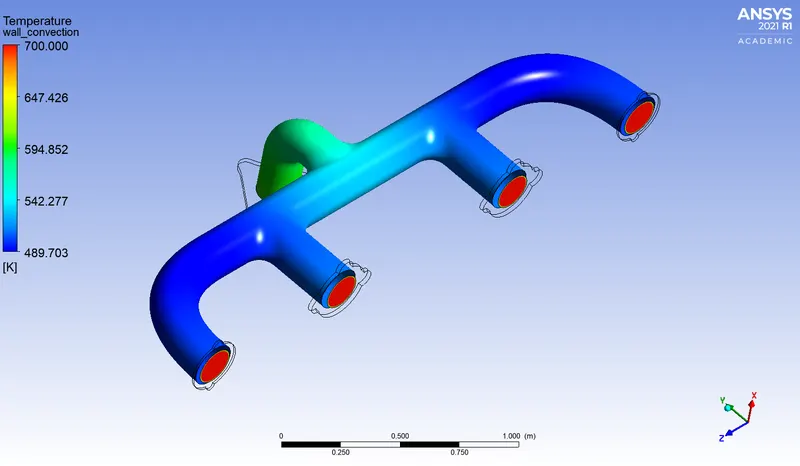
It is observed that there is a regular trend in the residuals. The residuals of velocity and energy (main parameters) have residuals in the order of 1e-4 and 1e-6 respectively. In addition, it is found that the outer solid region temperature contour does not vary largely w.r.t. iterations (not shown). The final temperature contour is shown below. From these points of view, it can be said that convergence is attained.

II) Justification for the turbulence model used and Y+

The first inflation layer was created with an initial assumed Y+ of 60. The first cell height calculated with the Y+ calculator is only an estimate because the equation for the skin friction coefficient is an empirical correlation for a specific flow scenario (turbulent
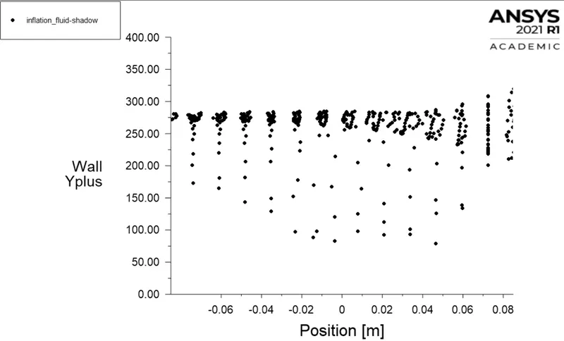
flow over a flat plate without an applied pressure gradient). With this assumption, the inflation layers were added in the fluid domain. Shown below is the plot of Y+ values in the 'inflation_fluid' named selection across the diameter of the inlets.

The Standard `k-epsilon` uses Y+ between 30 and 300. From the plot below, the majority of the cells have Y+ in the specified range and hence the turbulence model used is justified with the mesh.

III) Temperature Contours:

Temperature contour of Outer solid wall:

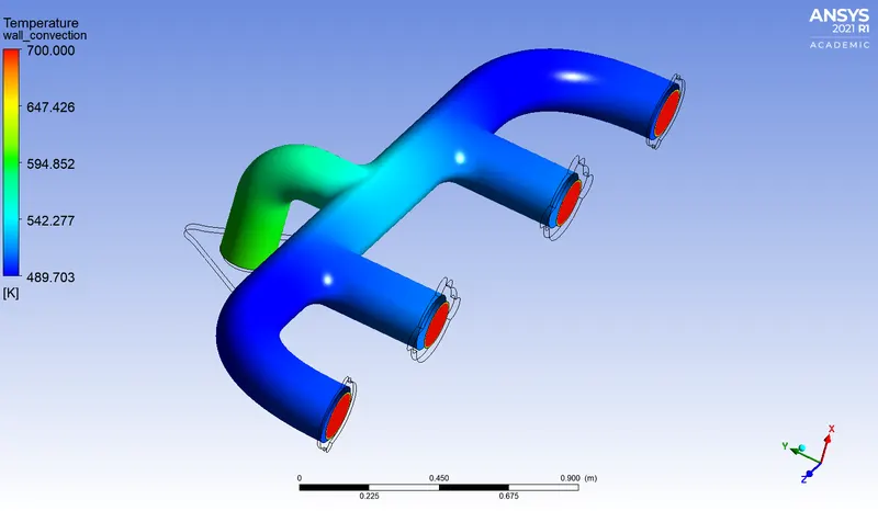
This temperature contour shows the temperature distribution at the Outer solid wall. The temperature distribution obtained at the inner solid wall is the same as the distribution obtained on the outer solid wall as conduction is neglected.

The temperature contour denotes that the temperature at the outer solid wall close to the outlet (~600K) is at a higher value than the temperature at the outer solid wall close to the inlet (~490 K). This result seems counter-intuitive at the first glance as hot air at 700K enters the Inlet and it makes sense if the temperature of walls close to the inlet is at a relatively higher temperature. To explain this result, the magnitude of the velocity of flow through the manifold should be looked at.

Streamlines & Velocity contour of flow through the manifold:

Through each inlet, hot air enters at 5 m/s. The geometry contains one outlet and all ports have the same diameter. Hence, from the law of conservation of mass, the velocity at the outflow must be greater than that of the inlet. The streamline plot shown below is colored by the velocity. It is observed that velocity drastically increases at the point where all the streams meet and the max velocity of ~ 40 m/s is obtained at the vertical pipe bend.

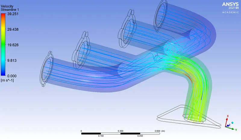
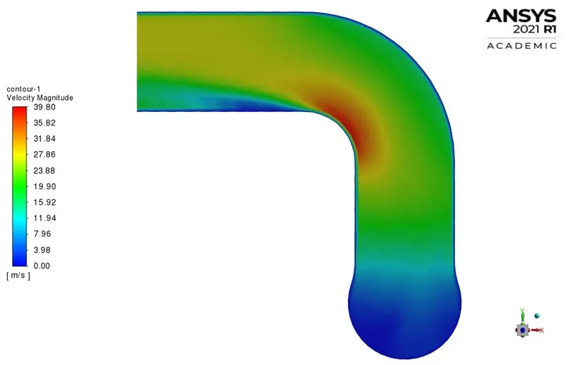
It is known that the HTC is dependant on the Nusselt number. The Nusselt number is a function of the Reynolds number and the Prandtl number. The Prandtl number is totally dependant on the material property and is a constant in this problem. Hence, the Nusselt number turns out to be maximum when the Reynolds number is maximum. This happens at the intersection of the inlet streams at the vertical pipe bend. Hence, the heat transfer from the fluid to the solid is maximum at this location. So, the temperature of the outer solid wall is maximum here.

Surface Heat Transfer Coefficient Contour:

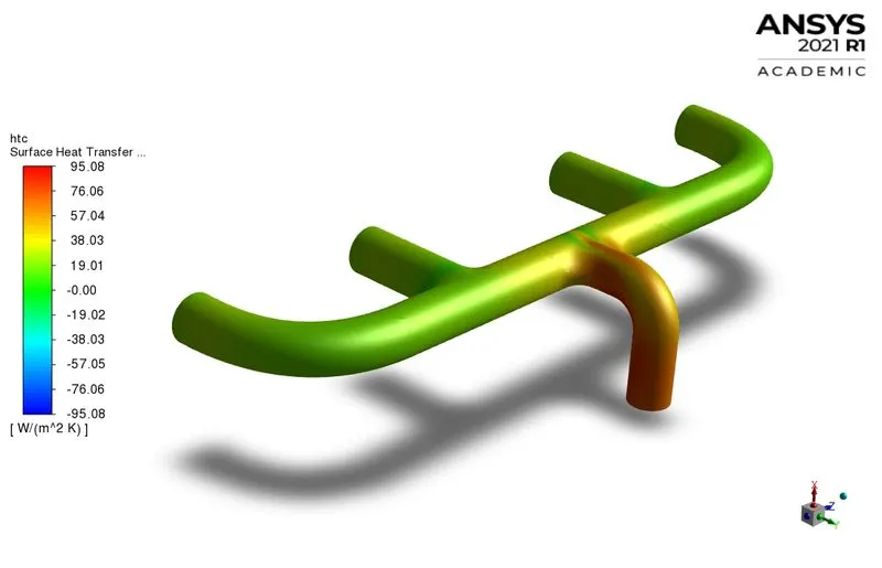
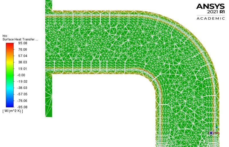
Shown below is the contour of the Surface HTC on the inner walls of the solid. As discussed in the previous sub-section, it can be concluded that the wall heat transfer coefficient is maximum at the solid inner wall close to the pipe bend. In the second image shown below, the mesh is visible. The heat transfer coefficient contour is visible along the solid-fluid interface at the wall. It attains the highest value ~95 `W/(m^2K)` close to the bend.

IV) Estimation and Comparison of Wall HTC:

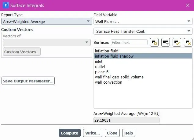
The area-averaged surface HTC is obtained over the inner solid surface using the Surface Integral option available under the 'Results' tab. The value is obtained is 29.19031 `W/(m^2K)`.

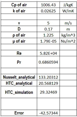
This result is compared using an analytical approach. For turbulent flow through a circular pipe, the Nusselt number is given by the Dittus Boelter Equation: `Nu = 0.023Re^0.8Pr^n`, where '`Re = (rhoVD)/mu`' is the Reynolds Number, '`Pr = (muCunderset(p)())/(kunderset(f)())`' is the Prandtl Number and n = 0.3 for cooling of fluid and n = 0.4 for heating of the fluid.

It is to be noted that the Dittus Boelter equation is valid for turbulent pipe flow. Here, the geometry is more complex as it involves multiple pipes with bends that are not accounted for in the Dittus Boelter equation. Hence, the HTC can only be compared and cannot be verified! Shown below is the calculation of analytical HTC. It is found to be equal to 20.568129. There is an error of -42.6 %. This can be attributed to the geometry (multiple pipes and pipe bends) and the mixing of different streams.

CONCLUSION:

Heat transfer is simulated from the flowing fluid to the solid region of the exhaust port. The inner wall HTC is estimated and compared with the analytical value. The temperature distribution on the solid wall is obtained. The counter-intuitive result obtained in the temperature distribution is explained.