Flow over Backward Facing Step using CONVERGE

OBJECTIVE:

The objective of this challenge is to set up a CFD simulation of flow through a Backward Facing Step using Converge. Backward Facing Step flow simulation serves as a benchmark problem in CFD for testing/validating the iterative solvers as a lot of experimental data is available. Sometimes the Backward facing step simulation is used to compute the efficiency of solvers.

SOFTWARES USED:

1. Converge Studio v3.0
2. Windows CMD and CYGWIN
3. Paraview

CASE SET-UP IN CONVERGE STUDIO:

In this challenge, the Backward facing step is constructed using triangle commands on Converge and a Steady-state simulation is run for three different mesh sizes and the results are compared. A steady-state solver is set up by monitoring the velocity obtained output cross-section.

1) Geometry:

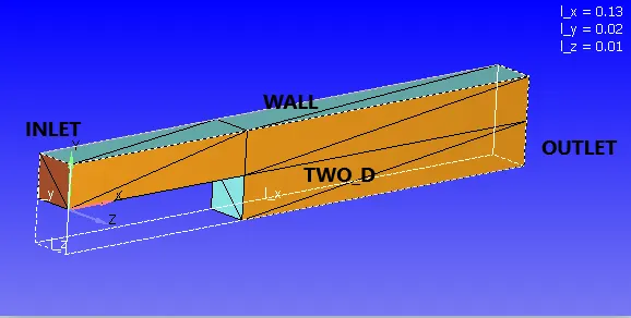
The dimensions of the geometry is 0.13m X 0.02m X 0.01 m.

2) Mesh:

The mesh sizes used in this challenge are:

CASE I) 2e-4 m in all three directions.

CASE II) 1.5e-4 m in all three directions.

CASE III) 1e-4 m in all three directions.

The main highlight of this simulation is the boundary layer separation phenomena followed by vortex formation as the flow undergoes sudden expansion. To capture the boundary layer information accurately, Mesh embedding is given to the geometry close to the step.

3) Material:

Gas ==> Air

4) Boundary Conditions:

The left and right surfaces have Inlet and Outlet boundary conditions respectively. The front and back are given the boundary condition of Two_D as the simulation is essentially 2D due to symmetry in the geometry. The top and stepped-bottom surfaces are given the condition of the Wall boundary condition.

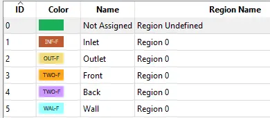
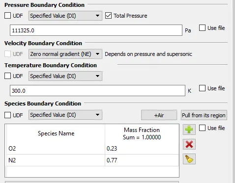
Inflow Boundary Condition: Total Pressure of 111325 Pa, Temperature of 300K, and Species of Air (O2 and N2) entering the channel.

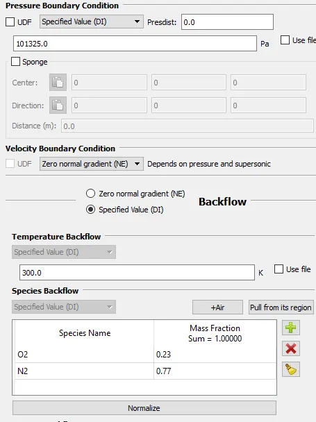
Outflow Boundary Condition: Static Pressure of 101325 Pa with species backflow as O2 and N2.

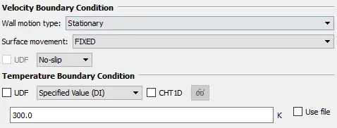
Top & Bottom: Wall Boundary Condition No-Slip Boundary condition is applied on Top and Bottom walls due to boundary layer formation and the temperature of the wall is set at 300K.

TWO_D Boundary Condition which means the simulation is essentially a 2D simulation and no equations are being solved on the 3rd axis.

5) Initial Conditions:

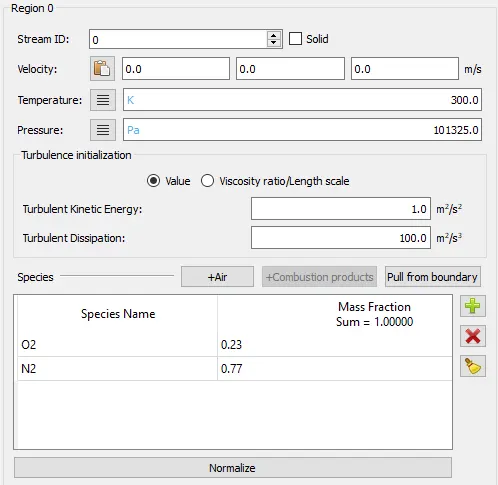
Species of Air (O2 of mass fraction 0.77 and N2 of mass fraction 0.23) present at 300K and 101325 Pa.

6) Simulation and Time parameters

A full hydrodynamic simulation is performed with a steady-state solver. Steady-state solver implies that irrespective of the path of the process and the initial conditions, the simulation will reach steady-state and give tangible results as long as the geometry and boundary conditions are given right.

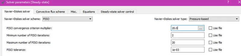
The N-S solver is set to PISO (Pressure Implicit with Splitting of Operators) which is predominantly used to handle unsteady simulations. It uses the concept of pressure correction; The algorithm uses 1 predictor step and 2 corrector steps to arrive at an accurate value for the pressure correction term.

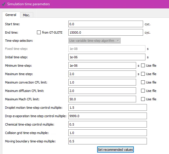
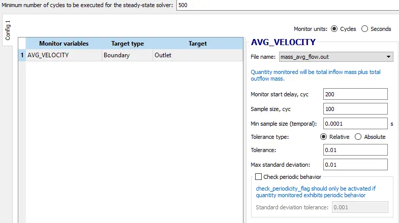
The time parameters and steady-state monitor are shown below: Simulation start time is 0 cycles and end time is 15000 cycles. It is controlled by a steady-state solver monitoring velocity at exit. The steady-state monitoring starts functioning after 500 cycles and once the average parameter (avg. velocity in this case) attains steady-state, the simulation is shut off. The average is calculated by taking sample data of a specified size (100 in this case). The relative tolerance limit set for a sample size of 100 cycles is 0.01.

7) Turbulence properties:

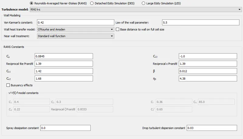
RNG `k-epsilon` turbulence model is set for the case. Generally, the standard `k-omega` SST model is used at the industrial level. Not many differences exist between RNG `k-epsilon` and the `k-omega` SST model.

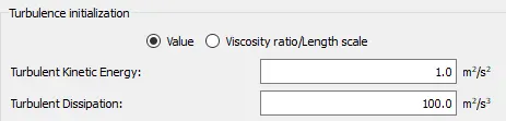
The (Initial Conditions) initial value of Turbulent Kinetic energy 'k' is assigned to the default value of 1 `m^2s^-2` and Turbulence Dissipation rate '`epsilon`' is assigned to the default value of 100 `m^2s^-3`.

The basic idea of the RNG `k-epsilon` model is to solve the transport equations involving Turbulent Kinetic energy 'k' and Turbulence Dissipation Rate '`epsilon`' to arrive at the values of k and `epsilon`. With the values of k and `epsilon`, the Eddy viscosity can be calculated. With the value of Eddy viscosity, the Reynolds stresses, and further, the RANS equation can be solved for average velocity. Shown below are the default RANS constants which are to be used in the k-`epsilon` transport equation.

8) Output/ Post processsing:

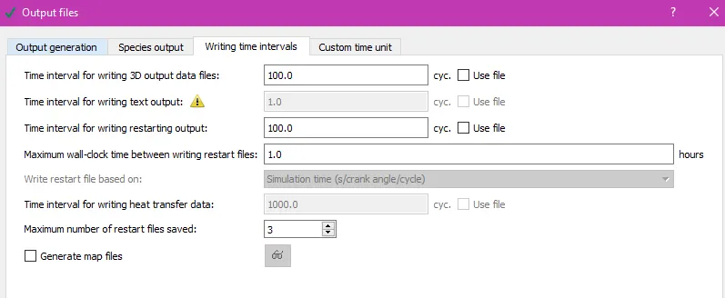
The post-run data variables selected are Pressure, Temperature, Velocity, and Density, Dissipation Rate (`epsilon`), Turbulent KE (k), Turbulent viscosity. The time interval of writing 3D Output files and text files are set such that 100 data files of each are generated. The time interval for restart files is the same as that of 3D output.

EXPORT OF INPUT FILES:

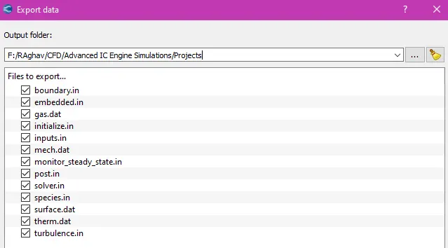
In Converge Studio, the case set-up of the problem is done. This essentially creates all the necessary input files for the Converge solver. Once the case setup is done, the input files are exported to a new folder. Shown below are the input files that have been generated by Converge Studio.

RUNNING THE SIMULATION:

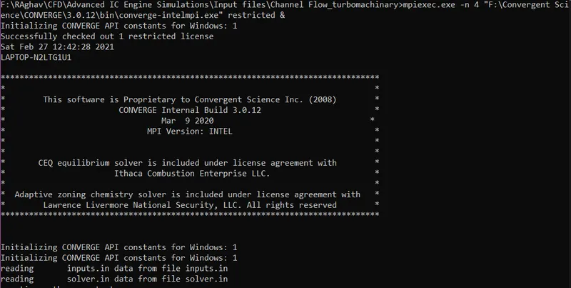
A Command-line editor tool like Windows CMD or CYGWIN is used to set up the run. Here Windows CMD is used. Firstly, the location of the input files is navigated to and the Converge solver is called using the Command Line tool. For faster computational speed, parallel processing is set up on 4 cores using INTEL MPI software.

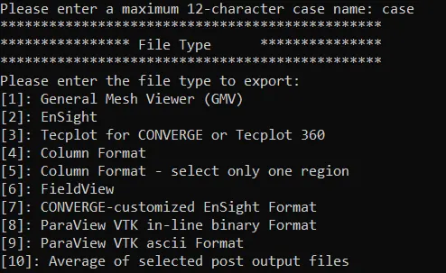
At the end of the run, the solver generates "post.h5" files (3D Output files) and ".OUT files" (Data files). The ".OUT" files contain data at mesh points. The 3D Output files are further post-processed using Converge post-processing tool into "Paraview VTK-Inline Binary format" to further analyze the case in Paraview.

RESULTS:

CASE 1) Mesh size: 2e-4 m

Mass Flow Rate Plot:

The initial oscillations in the plot are attributed to the transience in the problem. The mass flow rate converges to ~1.37 kg/sec at the Inflow Boundary. The mass flow rate converges to 1.37 kg/sec at the Outflow Boundary. The signs are not considered as the mass flow rate is positive.

Velocity Plot:

The initial oscillations in the plot are attributed to the transience in the problem. The velocity converges to 112.53 m/sec at the Inflow Boundary. The velocity converges to 58.15 m/sec at the Outflow Boundary. The signs are not considered as the velocity is positive. The decrease in velocity is attributed to an increase in cross-section area and Boundary Layer separation.

Pressure Plot:

Total Pressure at Inflow: 111325 Pa; Total Pressure at Outflow: 103673 Pa

Static Pressure at Inflow: 103391 Pa; Static Pressure at Outflow: 101325 Pa

Number of Cells:

Animation of Contours:

CASE 2) Mesh size: 1.5e-4 m

Mass Flow Rate Plot:

The initial oscillations in the plot are attributed to the transience in the problem. The mass flow rate converges to 1.5 kg/sec at the Inflow Boundary. The mass flow rate converges to 1.5 kg/sec at the Outflow Boundary. The signs are not considered as the mass flow rate is positive.

Velocity Plot:

The initial oscillations in the plot are attributed to the transience in the problem. The velocity converges to 120 m/sec at the Inflow Boundary. The velocity converges to ~65 m/sec at the Outflow Boundary. The signs are not considered as velocity is positive. The decrease in velocity is attributed to an increase in cross-section area and Boundary Layer separation.

Pressure Plot:

Number of Cells:

Animation of Contours:

Mesh size: 1e-4m

Mass Flow Rate Plot:

The initial oscillations in the plot are attributed to the transience in the problem. The mass flow rate converges to ~1.5 kg/sec at the Inflow Boundary. The mass flow rate converges to 1.5 kg/sec at the Outflow Boundary. The signs are not considered as the mass flow rate is positive.

Velocity Plot:

The initial oscillations in the plot are attributed to the transience in the problem. The velocity converges to ~120 m/sec at the Inflow Boundary. The velocity converges to ~62 m/sec at the Outflow Boundary. The signs are not considered as the velocity is positive. The decrease in velocity is attributed to an increase in cross-section area and Boundary Layer separation.

Pressure Plot:

Number of Cells:

Animation of Contours:

Boundary Layer Separation and its Effect:

At the step, the fluid flow experiences sudden expansion, due to which there is a separation of the fluid from the walls of the channel. This is called Boundary Layer Separation.

The boundary layer separation is a phenomenon that occurs when a fluid encounters a sudden change in cross-section in the path of the fluid flow. The necessary and sufficient conditions for boundary layer separation to occur are the Adverse (positive) pressure gradient and a zero velocity gradient normal to the flow.

The adverse pressure gradient is caused due to the change in cross-section. As the area of cross-section increases, the velocity decreases; as the velocity decreases, the pressure increases. This local increase in pressure causes a positive pressure gradient region where the net force on the fluid particles is opposite to the direction of flow. This force reduces the velocity of the fluid particles. Once the velocity near the wall becomes 0, flow reversal takes place and separation occurs.

This phenomenon is usually accompanied by vortex formation. Vortex consumes a lot of mechanical energy of the fluid and hence accompanied by a large local pressure drop and a massive increase in local velocity. Shown below is the formation of the vortex near the Step.

INFERENCES AND CONCLUSION:

1. The number of cycles that each mesh case runs is based on the transience of the problem and the tolerance and sample size that have been set in the solver. The problem is initially transient and the solver stops when a steady state is attained.
2. Mesh Embedding is used to capture the effects of Boundary Layer separation. It can be seen that the total number of cells in for the 2e-4m mesh size is ~1000 cells, ~1400 for 1.5e-4m mesh size, and ~3000 for 1e-4m mesh size. As the mesh size increases, there is an exponential increase in simulation time with an increase in the accuracy of the solution.
3. The RNG `k-epsilon` turbulence model is used.
4. In all three mesh cases, we can see that the mass flow rate is almost the same at Inlet and Outlet. The average velocity at the inlet is higher than the outlet due to loss of KE in boundary layer separation.
5. The static pressure is constant at the outlet boundary but decreases in the Inlet boundary. Similarly, the total pressure is constant at the Inlet boundary and increases at the Outlet boundary. The value of static pressure is higher at the outlet because, as the area increases, the static pressure increases. Similarly, the value of total pressure at the outlet is lesser than inlet as pressure this change in pressure drives the flow from left to right.
6. Near the step, a phenomenon of Boundary layer separation of the fluid takes place. The necessary and sufficient conditions for Boundary Layer separation are adverse pressure gradient and zero velocity gradient normal to flow. The effects of Boundary Layer separation are Vortex formation and loss in KE of fluid.