Simulating Combustion of Natural Gas using Fluent

OBJECTIVE:

To simulate combustion in a Combustor and plot the variation of the mass fraction of the different species using line probes at different locations of the combustor using Fluent. Emissions such as NOx and Soot are also plotted. The effect on the temperature and emissions onthe addition of water to fuel is studied.

SOFTWARE USED:

1. Ansys Fluent 2021 R1

THEORY:

Theory of non-premixed Combustion and Species Transport Equation:

Reference: ANSYS FLUENT MANUAL

The main difference between Premixed and non-premixed combustion is that the fuel and the oxidizer enter the reaction zone in distinct streams in the case of non-premixed combustion whereas reactants are mixed at the molecular level before burning in premixed combustion.

Fluent can model the mixing and transport of chemical species by solving conservation equations describing convection, diffusion, and reaction sources for each component species. To model Volumetric reactions (reactions occurring in fluid phase), such as in a combustor, Fluent follows two main approaches: i) Species Transport Equations and ii) The Generalized Finite-Rate Formulation for Reaction Modeling. The Species Transport approach is discussed in this section and is used to model the combustion in this challenge.

The Species Transport Equation:

The Species Transport equation is given by:

where `Yunderset(i)()` is the mass fraction of the 'i' th species, `Runderset(i)()` is the net rate of production of species by chemical reaction, and `Sunderset(i)()` is the rate of creation by addition from the dispersed phase plus any user-defined sources. This equation is solved for N-1 species. N is the total number of fluid phase chemical species present in the system. The mass fraction of Nth species is calculated using 1- the sum of the calculated mass fraction of N-1 species. Here `vec J underset(i)()` represents the diffusion flux of species i. The diffusion flux is a combination of Laminar or Turbulent species diffusion. Turbulent diffusion generally outweighs Laminar diffusion. For most engineering applications, flow is largely turbulent. In such cases, the Laminar diffusion coefficient can be neglected and the turbulent diffusion coefficient can be estimated using Dilute Approximation. The Dilute Approximation approach considers the diffusion of species i into the whole mixture based on the concentration gradient rather than diffusion from species to species. In the case of Laminar flow, there is a need for Multicomponent diffusion properties. This is a very costly method and is used only if needed.

The Combustion Source term is calculated in three ways based on the application.

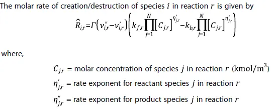
i) Finite Rate Chemistry:

In this approach, the effect of turbulent fluctuations on kinetics rates is neglected and reaction rates are determined by general finite-rate chemistry directly. This is a detailed chemistry solver and solves for the reaction rates of species from an ODE system obtained from the reaction mechanism. This is a more accurate model but is slow.

ii) Mixing Based Model:

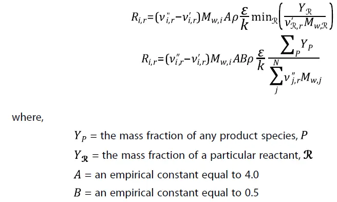
In certain engineering applications such as burners, combustion occurs when the mixing of air and fuel occurs in the right amounts. This mixing is driven by turbulence. The Eddy-Dissipation Model is a mixing-based model. Based on the values of k and `epsilon`, a Mixing Time Scale is calculated, after which combustion occurs. The chemical reaction rate is governed by the large-eddy mixing time scale,`k/epsilon`. Combustion proceeds whenever turbulence is present (`k/epsilon > 0` ) and an ignition source is not required to initiate combustion. This is acceptable in non-premixed combustion.

The net rate of production of species due to reaction r, `Runderset(i,r)()`, is given by the smaller, that is, the limiting value of the two expressions below:

iii) Finite Rate Eddy Dissipation Model:

Detailed chemical kinetics can be incorporated in turbulent flames, considering the timescales of both turbulence and kinetics. In premixed flames, the reactants will burn as soon as they enter the computational domain. To ensure this does not happen, Fluent provides the Finite-rate Eddy Dissipation model, where both the finite-rate reaction rates and eddy-dissipation and rates are calculated. The net reaction rate is taken as the minimum of these two rates.

GEOMETRY AND PHYSICAL MODEL:

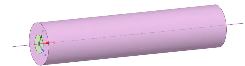
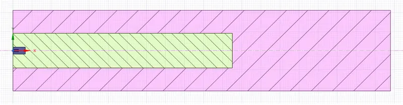
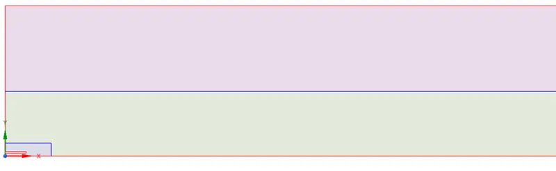
The geometry is a cylindrical combustor that burns in a co-flow air stream. The left side section of the combustor is the Inlet and the right side of the combustor is the Outlet. Non-premixed combustion occurs. The fuel is injected through a small cylindrical nozzle at high speeds in the middle of the Inlet. The air enters through the remaining section of the Inlet. As the geometry is axisymmetric, the computational domain is reduced to 1 degree. It essentially turns out as a 2D simulation that reduces the computational resources required as well.

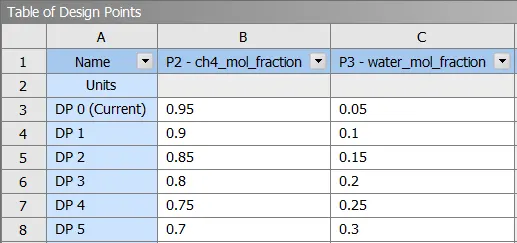
The fuel used is Natural Gas. The combustion is captured using Eddy Dissipation Model. The Combustion of natural gas in the combustor is investigated under two criteria in this challenge. In Case #1, 100% Natural gas (100% CH4) is used as a fuel. Emissions observed are Soot and NOx. In Case #2, the fuel used is a Fuel-Water Emulsion (FWE). The concentration of the water is varied from 5% to 30% by mole using a Parametric study. The effect of the addition of water to the fuel is observed on the temperature contours across the combustor and on the production of NOx and Soot.

The Combustor, its cross-section, and the reduced 2D axisymmetric geometry are shown below.

CASE SETUP IN ANSYS:

I) Geometry:

The 3D geometry is reduced to a 2D axisymmetric geometry by using the 'Splitbody' option ==> Copy Surface ==> Remove the part of the geometry that is symmetric about the X-axis. Shown below is the obtained 2D geometry. Now, the faces are shared in order to create a conformal mesh. The dimensions of the bounding box of geometry are 792mm X 85 mm X 0 mm.

II) Meshing:

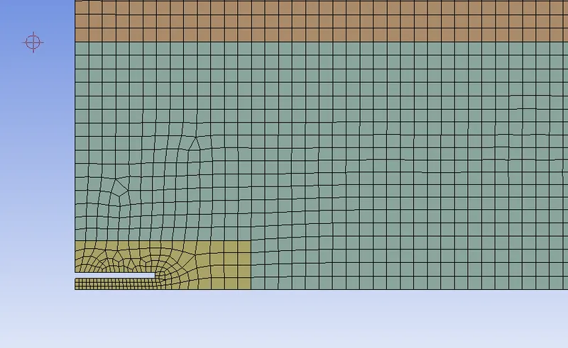
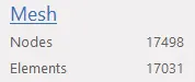
A structural mesh is generated by default by the Ansys Meshing. The base element size is set to 2mm. The 'Capture proximity' is enabled to define the minimum number of cell layers between gaps. It is set to a default value of 3. The conformal meshing, as well as the mesh close to the fuel injector gap, can be seen from the images below. Named selections Air_Inlet, Fuel_Inlet, Outlet, Walls, and Axis are made.

III) Fluent set-up:

• A pressure-based, steady-state solver is used. Axisymmetric is enabled in 2D Space.
• Under the Physics tab, the Energy equation is enabled. The Standard k-`epsilon` Model with Standard Wall function is enabled.
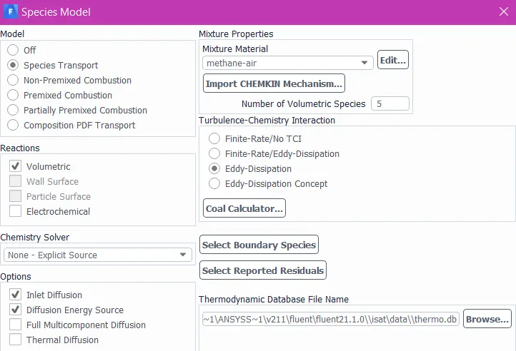
• Next, the Species button is clicked under Physical Models. The Species Transport option is checked. 'Volumetric reactions' is selected with Inlet Diffusion and Diffusion energy source enabled. The mixture material is selected depending on the case. In Case #1, methane-air is selected and in Case #2, methane-air-2step is selected. The turbulence-chemistry-interaction (TCI) is set to Eddy Dissipation. Additionally, the NOx emissions model is set to Thermal NOx and the Soot Model is set to the One-step approach.

• Next, the boundary conditions are defined. Air enters from the Air_Inlet at 0.5 m/s, at 300K with the following composition.

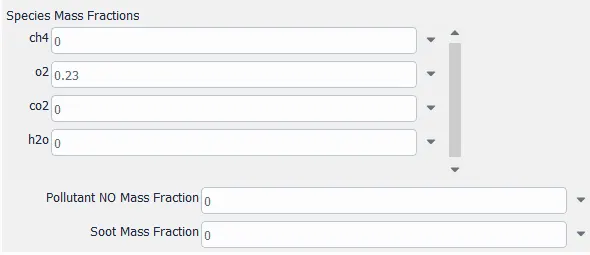
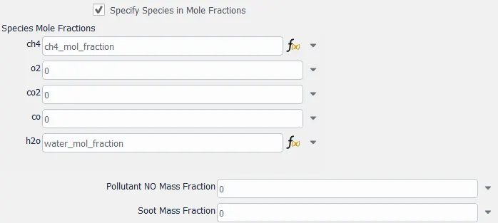
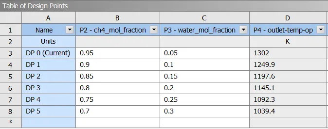
• Fuel enters at 80 m/s, at 300K with the composition as stated: Methane mass fraction = 1 in Case #1. In Case #2, the composition is specified by mole fraction. Methane and Water constitute the fuel composition and are set Input parameters. The input parametric table of design points is shown.

• The walls are specified constant temperature BC at a value of 300 K. The Outlet BC is set to 1 atm.
• An area-averaged value of static temperature at the Outlet C/S is assigned for reporting. An output parameter is created for this assignment. A temperature contour across the 2D plane is set up to visualize combustion. Solution animation of the temperature contour can be set if needed by the user.
• A Coupled scheme is set for the Pressure-Velocity Coupling. The discretization scheme of all the species involved is set to 'Second Order Upwind' by default.
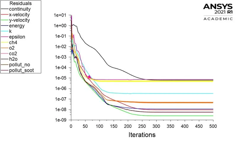
• The solution is initialized using the Hybrid solver. The number of iterations is set to 500 and the cases are run.
• Case #1 is run. In Case #2, one case is run from fluent (DP0) and the remaining cases are calculated from Workbench using the 'Update all design points' option.
• The temperature contours are analyzed in CFD-Post.

RESULTS:

1) Convergence:

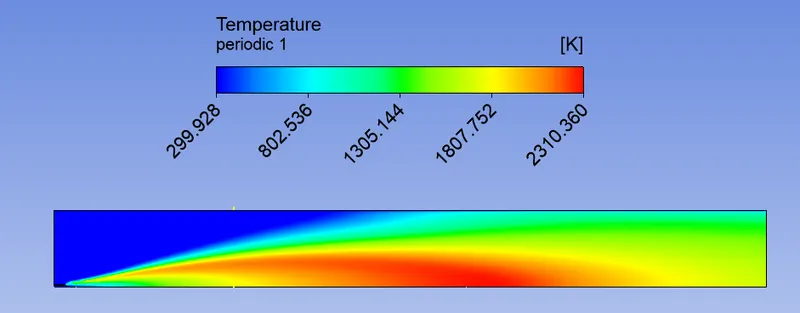
The residual plot is shown below for Case #1. The residuals become constant for all parameters around ~300 iterations. The temperature contour also does not change wrt iterations. It can be said that the solution has reached a pseudo-steady state. The same trend is observed for other cases.

2) Temperature Contour of the Combustor (Case #1):

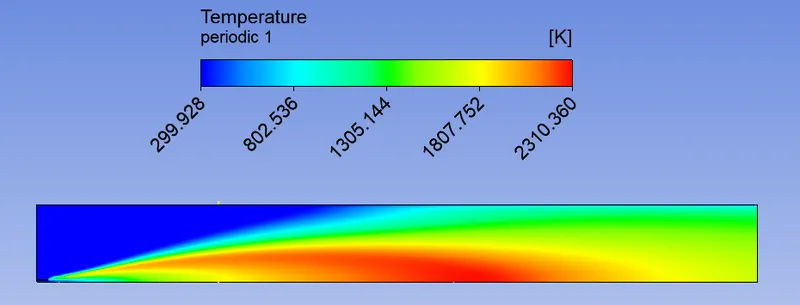
• Shown above is the temperature contour of the combustor. The different contour lines also represent the flame front produced.
• The area-averaged temperature at the outlet is 1355.137 K.

3) Mass Fractions Contours and Line plots of species across the probes (Case #1):

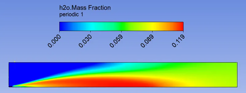
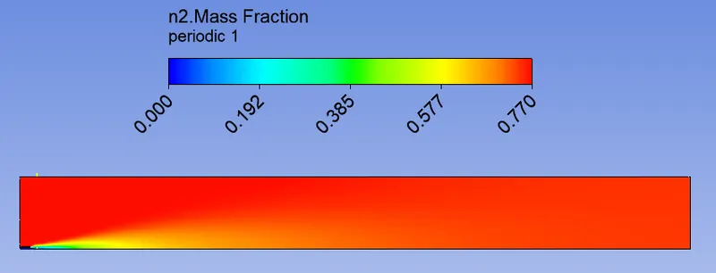
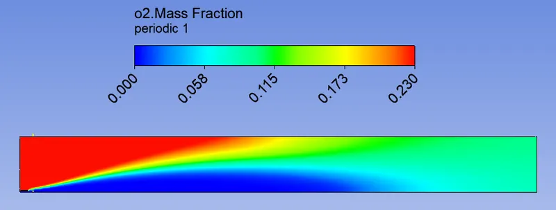
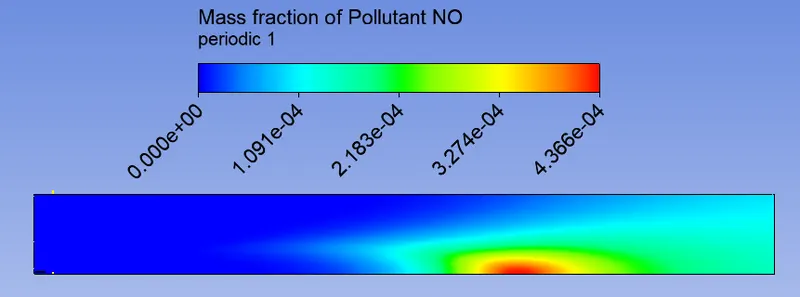
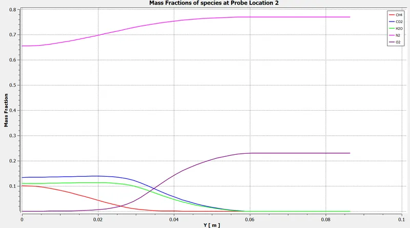
• Line probes are generated at various locations to observe the variation of species concentration across the probe.
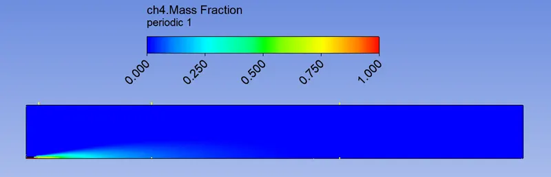
• The location of these probes is determined based on the species contours. For example, it is not wise to look at the mass fraction of CH4 species at the outlet of the combustor when it is being injected at the fuel_inlet.

i) Mass Fraction Contour of CH4:

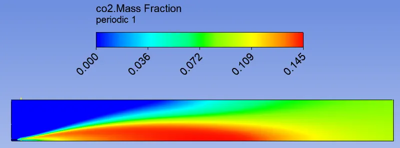
ii) Mass Fraction Contour of CO2:

iii) Mass Fraction Contour of H2O:

iv) Mass Fraction Contour of N2:

v) Mass Fraction Contour of O2:

vi) Mass Fraction Contour of NOx Emissions:

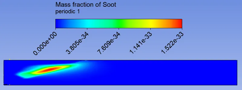
vii) Mass Fraction Contour of Soot Emissions:

viii) Variation of Mass Fractions of species across Line probe:

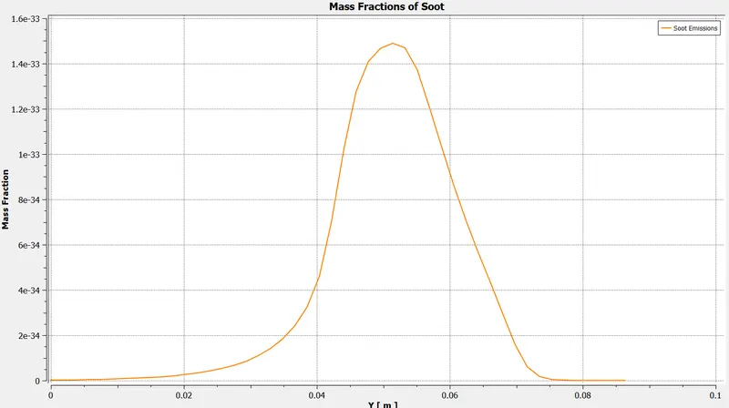
ix) Variation of Mass Fractions of Emissions across Line probes:

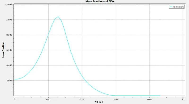
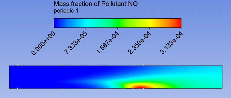
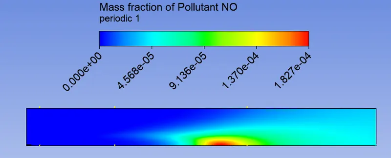
• The concentration of NOx emissions is maximum at the location where the temperature is maximum. From the contour, this location is observed to be somewhere close in the middle of the geometry. The NOx mass fraction is in the order of 10e-6.
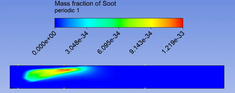
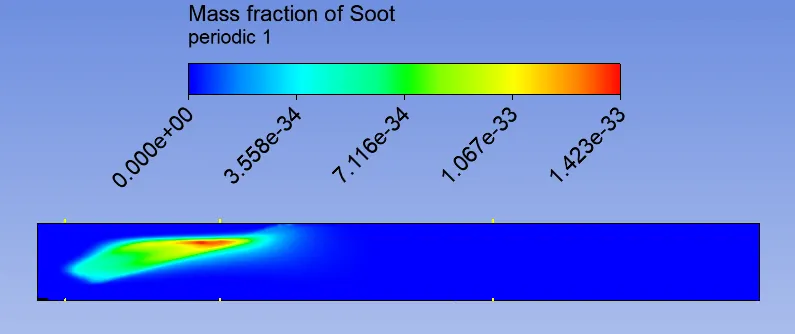
• Soot is formed as a result of incomplete combustion. From the soot contour, this region of formation is located just above the flame front close to the injector. Combustion does not occur here due to the high velocity at which the fuel is injected. Soot so formed is very less in concentration and its mass fraction is in the order of 10e-33.

4) Variation of Average Temperature at the Outlet of Combustor with the addition of water (Case #2):

• Historically Fuel-Water Emulsions (HWE) have been used in Marine engines to reduce the peak temperature of combustion and hence the emissions due to strict norms imposed by its regulations.
• The addition of water to fuel increases the ignition delay. In the extra time available, the fuel spreads into the chamber that results in more uniform mixing. This reduces the peak temperature obtained during combustion and hence the NOx emissions.
• It is known from theory the HWE results in better combustion and there is a reduction in NOx and Soot emissions.
• The effect of adding water to fuel on emissions is studied in the next section.
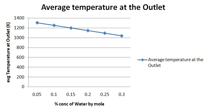
• The variation of area-averaged temperature at the Outlet is shown wrt increasing levels of water concentration by mole.
• A gradual reduction in the temperature is observed. The same is plotted that is shown below.

5) Effect of adding water to fuel on Temperature and Emissions (Case #2):

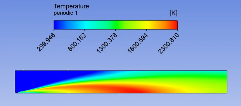
i) Temperature Contour at addition of 5% water by mole:

ii) Temperature Contour at addition of 15% water by mole:

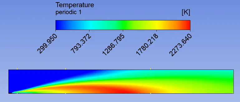
iii) Temperature Contour at the addition of 30% water by mole:

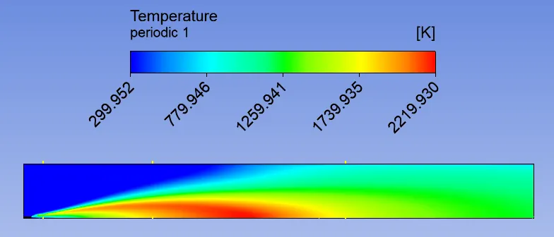
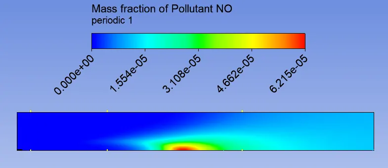
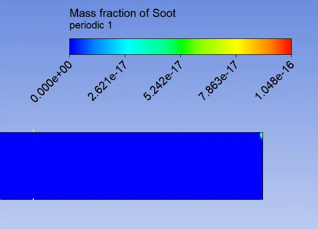
• With the addition of water, contour lines of temperature occupy a relatively smaller area in the contour. The max temperature attained decreases and the area-averaged temperature at the Outlet decreases.
• The region of NOx production shifts towards the left as there is a change in the location of the max temperature attained.
• The region of Soot production shifts towards the right. This can be attributed to the extra time available for the fuel to spread due to the addition of water. At and above 20% mole fraction of water addition, the region of soot production abruptly changes. It is observed at the top right corner of the geometry as shown in the above contour. In all other zones, the soot mass fraction is observed to be 0.

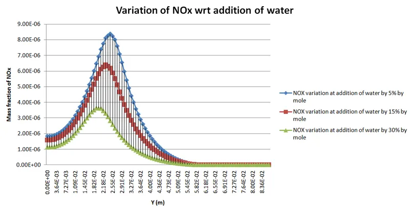
iii) Line probe comparison of the variation of Emissions with the addition of water:

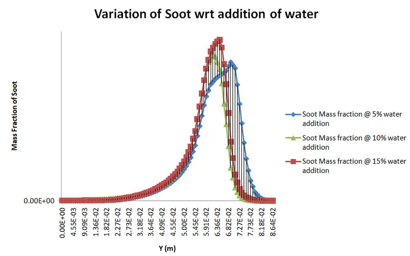
• The soot concentration increases with the addition of water as a result of incomplete combustion.
• At and above the water mole fraction of 20%, the Soot mass fraction is found to be 0 at the probe location, as the region of generation of soot abruptly shifts towards the outlet. Its mass fraction is in the magnitude of 10e-35.
• The NOx concentration decreases gradually with the addition of water. Its mass fraction is in the magnitude of 1e-6.

CONCLUSION:

1. Combustion in a combustor simulated using Turbulence Chemistry Interaction based Eddy Dissipation Model.
2. Temperature contours and line plots of mass fraction of species are observed along line probes.
3. The addition of water to the fuel decreases the average temperature.
4. The addition of water to the fuel decreases NOx emissions but increases Soot emissions.

References:

1. An overview of systems supplying water into the combustion chamber of diesel engines to decrease the amount of nitrogen oxides in exhaust gas; Leszek Chybowski, Rafał Laskowski, Katarzyna Gawdzinska
2. Modelling soot production and thermal radiation for turbulent diffusion flames; Lorenzo Mazzei, Stefano Puggelli