Simulating Cyclone separator with Discrete Phase Modelling using Fluent

OBJECTIVE:

To perform a CFD analysis on a Cyclone Separator using the Discrete Phase Modelling (DPM) approach. The inlet mixture is a combination of Air and Anthracite particles. The discrete particle Separation Efficiency and the pressure drop that occurs across the separator are to be calculated.

SOFTWARE USED:

1. Ansys Fluent 2021 R1

THEORY:

i) Discrete Phase Modelling (DPM):

Reference: ANSYS FLUENT MANUAL

Currently, there are two ways to model multiphase flows: The Euler-Lagrange approach and the Euler-Euler approach. In the Euler-Euler approach, the different phases are treated mathematically as interpenetrating continua and the sum of volume fraction of all the phases in a computational cell is 1. The Euler-Euler approach includes the methods such as the Volume of Fluid method, the Mixture method, and the Eulerian model.

The Discrete Phase Model in Fluent follows the Euler-Lagrange approach. In the Euler-Lagrangian approach, the fluid phase is treated as a continuum and the Navier-Stokes equations are solved in the continuum, while the dispersed phase is solved by tracking a large number of discrete particles through the calculated flow field. This dispersed phase can exchange momentum, mass, and energy with the fluid phase. An important assumption in this modeling is that the volume fraction of the discrete phase is very small (<0.1).

For calculating the trajectories of the discrete particles, Fluent integrates the force balance on particles in a Lagrangian reference frame. Shown below is the force balance equation. The particle trajectories are computed individually at specified intervals during the fluid phase calculation. This is represented by the flowchart shown below.

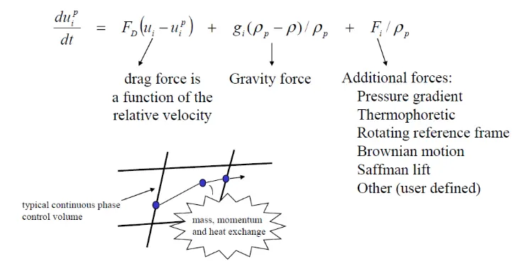
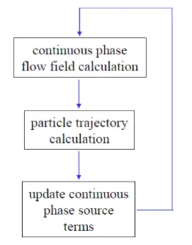
Additionally, in Fluent, the user has the option to explicitly define the type of coupling between the continuous phase and the discrete phase. A one-way coupling means that the fluid phase influences the discrete phase due to its drag and turbulence but the discrete phase does not influence the continuous phase. The two-way coupling means that the fluid phase influences the discrete phase due to its drag and turbulence and in turn, the discrete phase also transfers mass, energy, and momentum to the continuous phase. Both the phase equations are solved alternatively until the solutions stop changing in both phases.

Tracking Parameters in Fluent:

i) The Maximum number of timesteps:

The Maximum number of timesteps is used to find whether a given particle keeps recirculating in a particular region of the continuous flow phase. After the specified max number of timesteps, fluent stops tracking a particular particle and reports its trajectory as 'incomplete' meaning that the discrete particle is present in a recirculating region of the continuous flow.

ii) Length Scale:

Length scale controls the integration time step size in the particle equation of motion. The length scale is equivalent to the distance that the particle will travel before its motion equations are solved again and the trajectories are updated. The integration time step is directly proportional to the specified Length Scale and inversely proportional to the sum of velocities of the continuous phase and the discrete phase. A smaller value of the length scale yields accurate results.

iii) Step Length Factor:

The step length factor is another parameter specified to control the integration timestep size of the particle equation of motion. Step length factor can be specified instead of the Length Scale. This option allows fluent to compute the step size in terms of the number of timesteps required for a particle to traverse a computational cell. The integration time step size is computed by Fluent based on a characteristic time that is related to an estimate of the time required for the particle to traverse the current continuous phase control volume. If this estimated transit time is defined as`trianglet^star`, Fluent chooses a time step size as `triangle t = (trianglet^star)/(lambda)`where `lambda` is the step length factor. A larger value for the Step Length Factor decreases the discrete phase integration time step size and hence yields more accurate results.

ii) Flow behavior in a cyclone separator:

REFERENCES:

• Numerical study of gas-solid flow in a cyclone separator, B. Wang, D.L. Xu, K.W. Chu, A.B. Yu
• Rankine Vortex

Cyclonic separation is a method of removing particulates from an air, gas, or liquid stream, without the use of filters, through vortex separation. Conventionally, predicting the flow field in a cyclone has been an empirical one. In the age of CFD, flow and turbulence predictions have been found to be very sensitive to the turbulence model because of the formation of a forced vortex in the separator. The three turbulence models widely used for cyclone simulations are `k-epsilon`, Algebraic stress model (ASM), and Reynolds Stress Model (RSM).

The `k-epsilon` model assumes isotropic turbulence meaning rotation and buoyancy is not important. But cyclones are anisotropic where rotation and buoyancy suppress vertical motions. ASM has difficulties predicting rotational flows. RSM does not make any assumptions on isotropic turbulence and solves transport equations for each component in the Reynolds stress and is the most accurate model for cyclone simulations. However, to reduce the computational effort, the RNG `k-epsilon`model can be used. It has been found from the theory that there exists about a 12% deviation on experimental data.

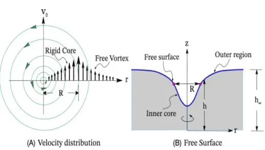
A Rankine-type vortex is formed in the cyclone separator. The Rankine vortex consists of a rigid core with an irrotational vortex in the far-field given by the image on RHS shown above. The region characterized by a radial distance r<=R corresponds to a rigidly rotating core while the outer region becomes a free vortex. At the same time, for a radial distance r>R">r>R, the model reverts to a free vortex, which allows for the velocity to decay at large distances.

The different flow components of flow and their behavior in the cyclone separator are mentioned below:

• The static pressure decreases radially from center to wall.
• The tangential velocity is zero at the walls and at the center of the separator.
• There exists axial velocity in the separator. That there exists both upward and downward flow depending upon the location of the vortex core.
• As far as radial velocity is concerned, it changes direction depending on the side of the vertical axis. It is positive on one side and negative on the other. The vortex rotates together with the flow around the geometric axis of the cyclone and has a helical structure.
• The resultant of the radial and axial velocity at certain locations build the way for a secondary recirculating zone that reduces the separation efficiency.

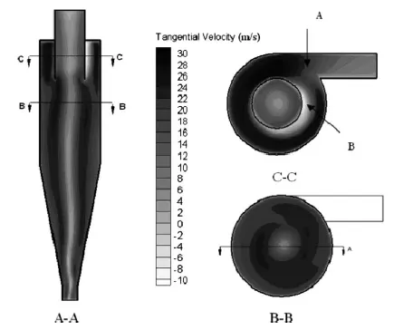
Shown below are images of the typical velocity distributions in a cyclone separator. The fourth image represents the locations of the secondary circulation region.

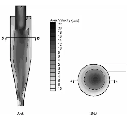
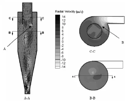
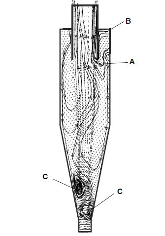
iii) Empirical Methods for the calculation of separation efficiency:

REFERENCE:

• A CFD Study on the Prediction of Cyclone Collection Efficiency; Jolius Gimbun, Thomas S. Y. Choong, T. G. Chuah, and A. Fakhru’l-Razi

As mentioned before, the study of flow in cyclone separators was conventionally an empirical one. Shown below are four empirical methods of finding the separation efficiency.

a) Iozia and Leith Model

This model is based on force balance. A particle carried by the vortex in the cyclone experiences two forces: Centrifugal force and Flow resistance. The collection efficiency `etaunderset(i)()` of particle diameter `dunderset(p i)()` is given by:

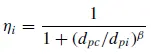where and `dunderset(pc)()` is the 50% cut size.

b)Li and Wang Model:

This model includes particle re-entrainment and turbulent diffusion at the cyclone walls. An assumption made in this model is that the radial particle velocity and the radial concentration profile are not constant for uncollected particles within the cyclone. The concentration distribution is given by:

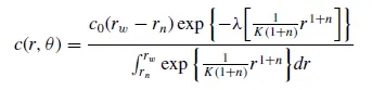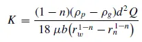where and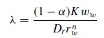

Now, the efficiency is calculated from where

c) Koch and Licht Model:

In this theory, the inherent turbulent nature of cyclones and the distribution of the particle residence times are recognized. Additionally, two assumptions are made: i) The tangential velocity of a particle is equal to the tangential velocity of the gas flow, ii) The tangential velocity is related to the radius of cyclone by: `uRoverset(n)()` = constant. The force balance equation and the particle distribution equations are used to find an expression for collection efficiency.

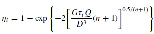where G is a factor related to the configuration of the cyclone, n is related to the vortex and `tau underset(i)()` is the relaxation term.

d) Lapple Model:

This model is based on force balance without the consideration of flow resistance. According to Lapple, a particle that travels from the inlet half-width to the wall in the cyclone is collected with 50% efficiency. The semi-empirical relationship to calculate the 50% cut diameter is given by 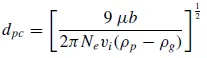where `Nunderset(e)()` is the number of revolutions. The collection efficiency is given by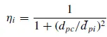

GEOMETRY AND PHYSICAL MODEL:

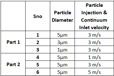
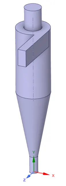
Shown below is the geometry of a cyclone separator. The fluid volume is extracted and a CFD analysis is run on the fluid volume to estimate the separation efficiency and pressure drop under varying inlet speeds of the mixture and varying diameters of the discrete particle. In this challenge, the separation efficiency is estimated by a rather general and intuitive expression given by the Number of particles trapped / the Number of particles tracked. Practically, it is known that high-efficiency cyclone separators deal with discrete particles above sizes of 2.5 `mum` in diameter. Hence the particle sizes considered are in the range of 1 `mum` to `5 mum`. The different cases that are to be simulated are listed below:

CASE SETUP IN ANSYS:

I) Geometry:

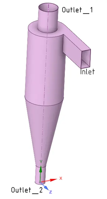
Shown below on the LHS is the 3D geometry of a cyclone separator. The fluid volume is extracted from the geometry and is represented by the RHS image shown below.

==>

II) Meshing:

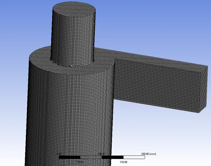
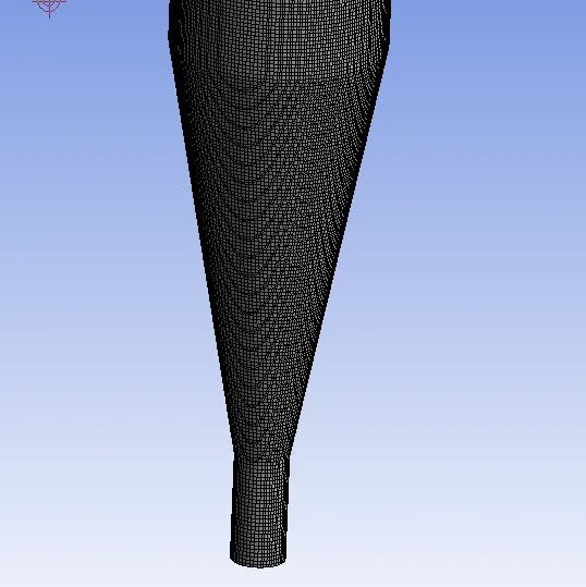
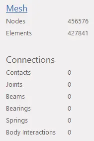
Structural mesh gives relatively better results. A body-fitted Cartesian mesh method is applied. The element size is specified as 5mm. Named selections such as Inlet, Outlet_1 (top) and Outlet_2 (bottom) are made.

III) Fluent set-up:

• A pressure-based, steady-state solver is used. Gravity is enabled with -9.81 m/s^2 in the Y direction.
• The RNG`k-epsilon` with Swirl Dominated Flow option turbulence model is selected.
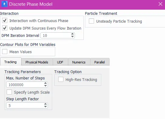
• The Discrete Phase Model is enabled. The two-way coupling is enabled. The DPM source term is enabled to update every iteration. The DPM iterations (force balance and trajectory calculation) are to be calculated every 10 iterations. The tracking parameters are varied according to the case. The step length factor is specified as the default value of 5.

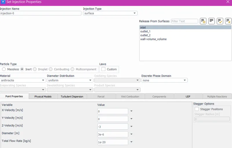
• Next, the discrete phase particle injection parameters are to be specified. The surface injection method is selected and the injection surface is selected as the named selection 'Inlet'. The discrete material that is to be injected along with the continuous phase is selected as 'Anthracite'. Its diameter and velocity are specified as per the case.

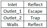
• The boundary conditions are specified next. The inlet velocity is specified as per the case. The outlet pressures are set to 1 atm. Additionally, boundary conditions are specified for DPM. They are given as follows:

• The solver scheme is set to Coupled Pressure-velocity coupling. The second-order upwind discretization scheme is set for the turbulence parameters k and `epsilon` as it is a turbulence-dominated flow.
• Next, the solution is initialized using Standard Solver. The case is then run for 600 iterations.
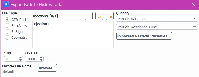
• After the solution converges, the particle history data file is to be exported in .xml format that is to be readable by CFD-Post for post-processing. This is done by File ==> Export ==> Particle History Data

RESULTS:

1) Convergence:

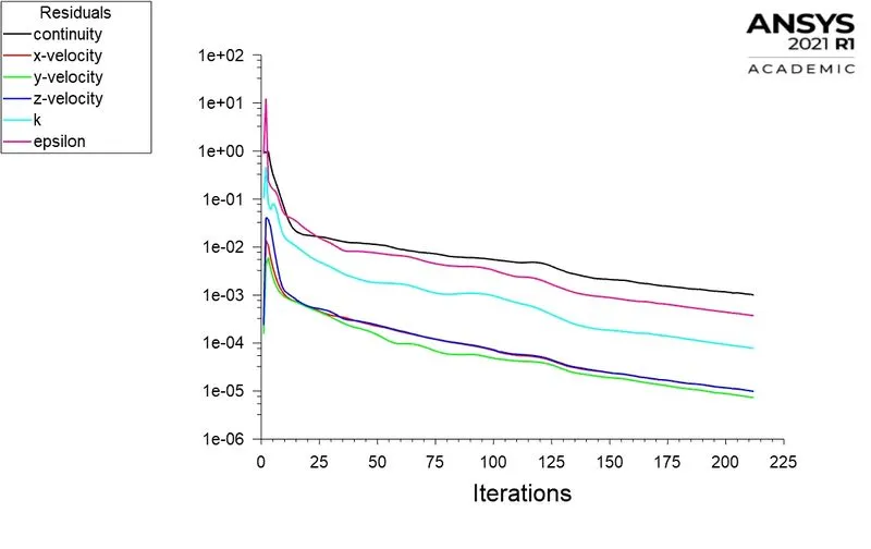
The residual plots are shown below. The solution attains a steady-state in ~250 iterations. The same trend is followed in all 6 cases.

2) Particle Trajectory and Residence Time Contour:

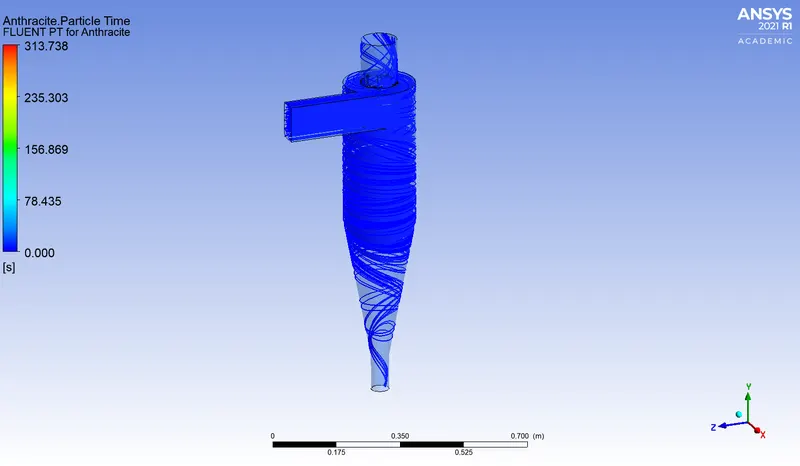
To visualize the trajectories of the particles in CFD-Post, File ==> Import ==> Import FLUENT Particle Track File ==> Select the saved file. Shown below is are the typical trajectories of discrete particles in the cyclone separator for Case #2 (3`mum` dia with 3m/s). The trajectories are colored by the particle residence times. It can be inferred that most of the trajectories are colored by dark blue meaning that the particle does not stay for longer times in the recirculation region and moves out of the zone.

A similar trend is observed for all other cases.

3) Separation Efficiency and Pressure Drop:

The DPM Iteration data for all 6 cases are shown below. It is noticed that the number of DPM iterations has been increased with reducing particle diameter. This is due to the fact that as the particle size decreases, the tendency for it to escape increases. Ideally, the number of particles that have incomplete trajectories must be close to 0. More particles must be trapped for more separation efficiency. To ensure the results obtained are steady, the DPM iterations are increased to ensure the correct number of the predicted Incomplete trajectories. The same strategy is used with decreasing velocity.

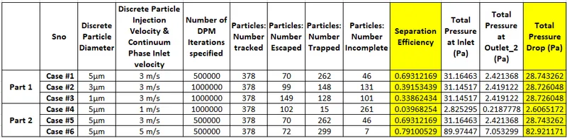
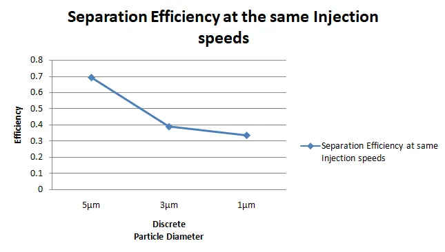
• It can be observed that, with decreasing diameter of the particle, at the same speeds, the separation efficiency decreases. This is because small particles tend to escape easily and do not get trapped. However, the size of the particle does not affect the total pressure in the system. The total pressure drop across the system remains constant.
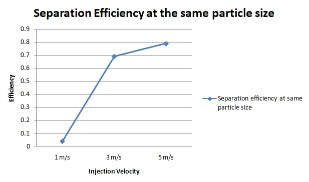
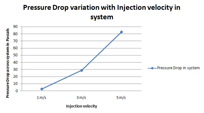
• With increasing injection speeds, at the same size of the particle, the separation efficiency increases drastically. This may be due to the increased strength of the forced vortex. But it is also observed that there is an abrupt increase in the pressure drop across the system as well. More external work would be required in order to keep the system running in this case.
• It is also to be noted that the separation efficiency also depends on the location of the inlet at which the particle enters the cyclone separator which is not discussed in this challenge. To further increase the separation efficiency in this system, the inlet dimensions of the separator have to be modified.
• The data values in the table are now represented by the line plots shown below.

4) Visualizing the Vortex Core:

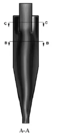
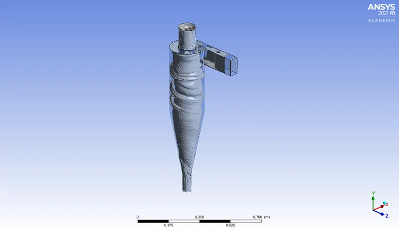
The vortex generated inside the separator is visualised from CFD-Post by Location ==> Vortex Core Region ==> Specify vortex strength. The vortex shown below can be related to the contour plots of the velocities shown in the initial section. The image of the typical tangential velocity in the separator is redisplayed for better visualization. The dark core present on the contour on the left is the vortex core itself. The velocity magnitudes change in the inner and outer regions.

CONCLUSION:

The Discrete Phase Model (DPM) is used in the simulation of the mixture of air (continuous phase) and Anthracite particles (discrete phase) through a cyclone separator. The Anthracite particles are separated from the mixture by the separator. The Anthracite particles are tracked and their trajectories are estimated. The separation efficiency is calculated by varying the diameter of the particles as well as varying the velocities. It is found that separation efficiency decreases with a decrease in the diameter of the particle and the separation efficiency increases with an increase in velocity at the inlet. But with an increase in efficiency, the total pressure drop across the system increases drastically as well.