Simulation of mixing of two fluid streams in a Mixing Tee using Fluent

OBJECTIVE:

In this challenge, the turbulent mixing of two streams of fluid is to be simulated and studied in a mixing-Tee geometry. The primary aim is to run different cases and come up with the effects of using a higher momentum ratio and a longer Tee. The effectiveness of mixing is to be determined at various physical conditions.

SOFTWARES USED:

1. Ansys Fluent 2021 R1

MIXING TEE AND ITS SIGNIFICANCE:

The mixing tee is a 'T' shaped junction. Two different streams at different temperatures of the same fluid enter through two inlets. The flow is turbulent and the mixing of the two steams happens primarily due to mixing. The resulting mixture having a resultant enthalpy at a resultant temperature leaves the Tee and is used for the required application. For example, the AC unit supplies air at a colder temperature than required where its operating efficiency is maximum. A mixing tee is required to bring up the temperature to the desired temperature.

The mixing in the 'T' is primarily due to the velocities flow field i.e., the turbulence. The parameter that characterizes the effectiveness of mixing is the standard deviation of temperature at the outflow boundary. Hence, the same will serve as the primary parameter in choosing the turbulence model, the convergence criteria, and grid independence criteria in this challenge.

GEOMETRY:

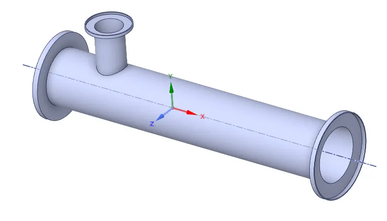
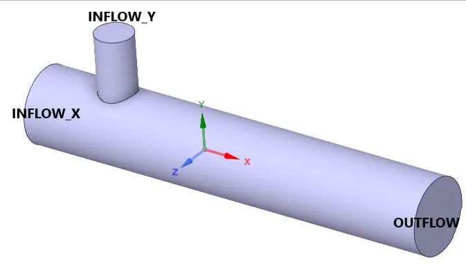
Two mixing tees are used in this challenge. One of them is longer than the other. The geometry of the Tee is shown below. The fluid volume is extracted and the boundaries are flagged using Named selections. The Inflow_X admits the hot stream and the inflow_Y admits the cold stream. The diameter of Inflow_X and Outflow is ~33.67 mm and that of Inflow_Y is ~16.9mm. The length of the shorter tee is 192.38 mm and the longer one is 268.33 mm

MESH:

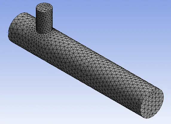
The mesh selected for the case is tetrahedral and the base mesh size is ~0.005 m.

CASE SET-UP IN ANSYS FLUENT:

a) Physics of the problem:

• Pressure based steady-state solver is used for the simulation.
• Energy solver is enabled as the problem is a thermodynamic problem.
• RANS-based Realizable `k-epsilon` and `k-omega` SST turbulence models are employed and based on the standard deviation on temperature obtained, one turbulence model is chosen for further analysis. This test is conducted on Case 1.1
• The material (fluid) is chosen as air.
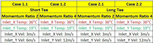
• The boundary conditions are specified as per the different cases shown below.

b) Solution and Simulation:

• Monitoring parameters such as Area averaged temperature at the outflow boundary and Standard Deviation at the outflow boundary are set up before starting the simulation. These plots are enabled for plotting.
• The case is initialized using the hybrid method. The hybrid initialization method uses a potential flow solver to come up with initial values for pressure and velocity.
• The number of iterations is set to 500 and the case is run.
• The results are discussed in the next section.

RESULTS:

a) Turbulence Model:

Case 1.1 was run with the Realizable `k-epsilon` and `k-omega` SST turbulence models.

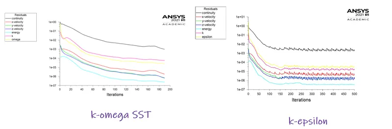
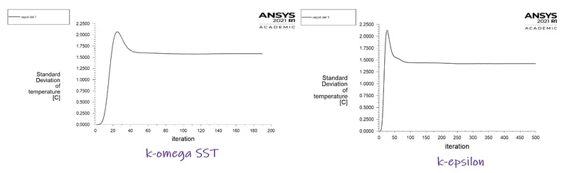
• The case with the Realizable `k-epsilon` does not satisfy the convergence tolerance and the simulation does not stop automatically. But from the residual plot, the same patterns of residuals keep repeating after 300 iterations. The `k-omega` SST case converges at 190 iterations.
• It is observed that the Realizable `k-epsilon` model generates the case at a standard deviation of slightly lesser than 1.5 Celcius where the `k-omega` SST model generates the case with a standard deviation of ~1.62 Celcius.
• The `k-omega` SST model is a shear stress transport model and captures the details close to the wall with greater accuracy by employing a distance from the wall-based formulation. But since this problem simulates the mixing effect away from the wall, the SST model cannot bring out its best results. The standard deviation of the Realizable `k-epsilon` is lesser than `k-omega` and is chosen as the turbulence model for further study.

b) Cell Count, Number of iterations for Convergence, Average Temperature at Outflow Boundary:

The following are the results obtained for the 4 cases.

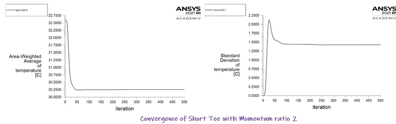
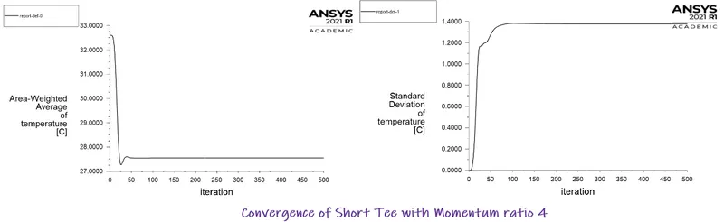
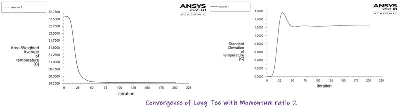
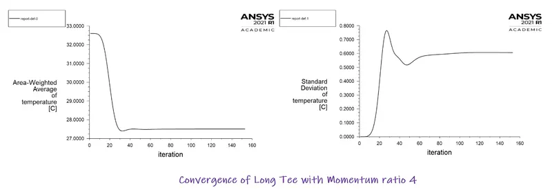
• With the increase in the momentum ratio, keeping the length of the tee constant, the average temperature obtained at the outflow boundary decreases. This is because, with higher velocity, the cold stream penetrates further into the hot stream and accelerates the turbulent mixing. Mixing happens primarily due to velocity.
• Increasing the momentum ratio significantly reduces the standard deviation of temperature at the outflow boundary indicating better mixing. The temperature profile obtained at the outflow boundary completely changes by doubling the momentum ratio. This will be shown later.
• By increasing the length of Tee, for the same momentum ratio, the average temperature at the outflow does not change significantly. But, the mixing process becomes more predictable and temperatures across the cross-section of the outflow boundary show lesser standard deviation.

c) Contour and Line Plots of Temperature and Contours of Velocity :

i) Short Tee with Momentum ratio 2

ii) Short Tee with Momentum ratio 4

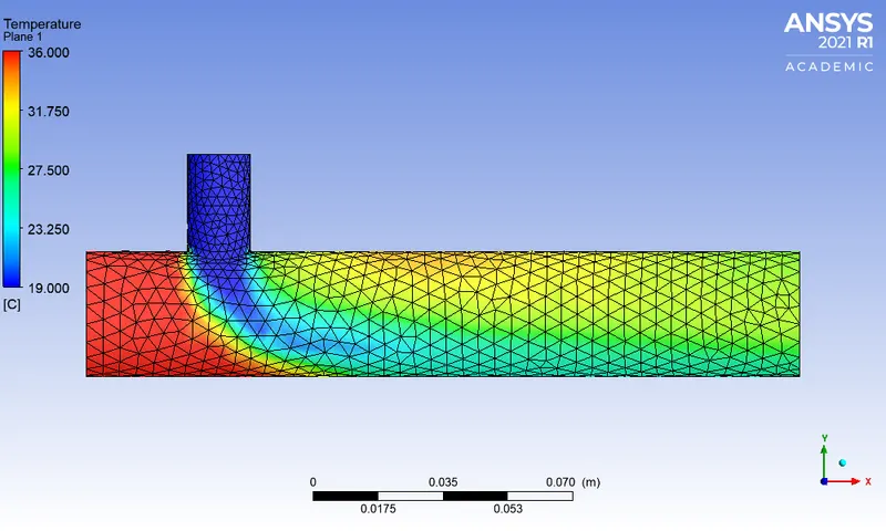
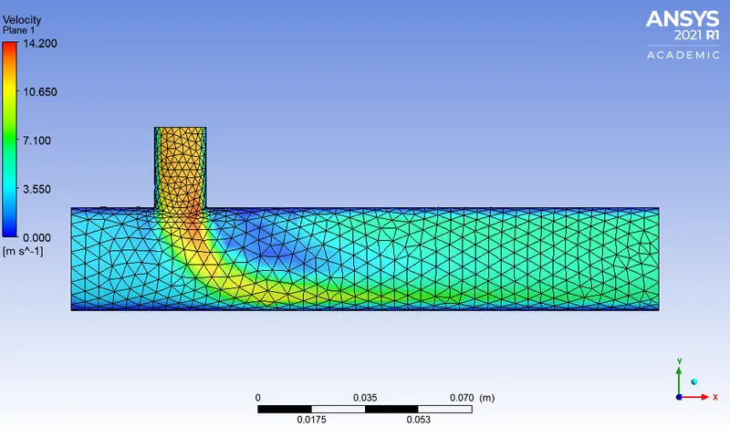
iii) Long Tee with Momentum ratio 2

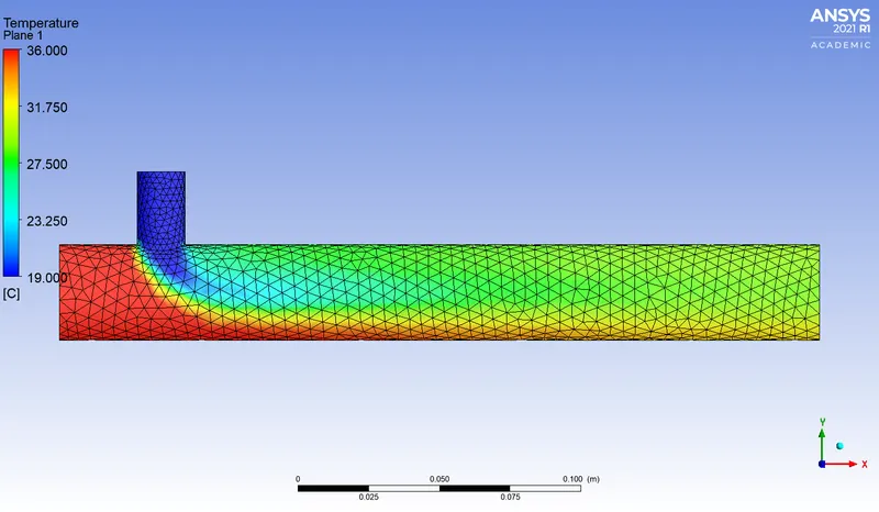
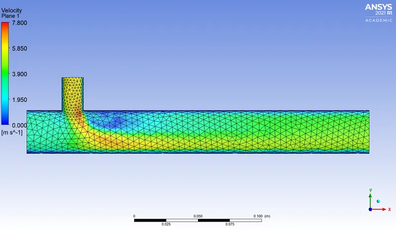
iv) Long Tee with Momentum ratio 4

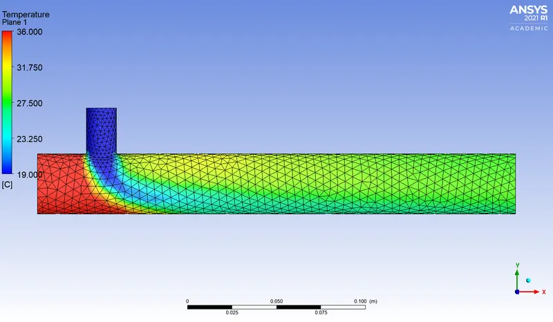
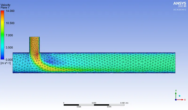
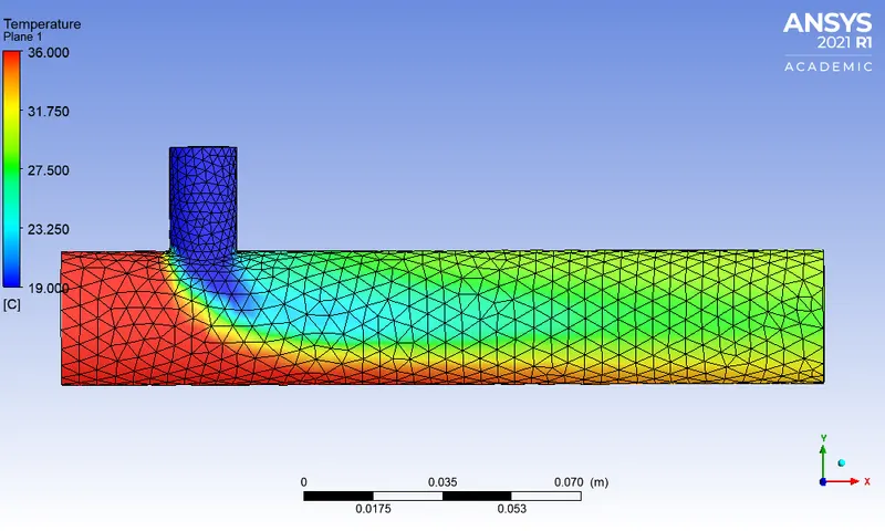
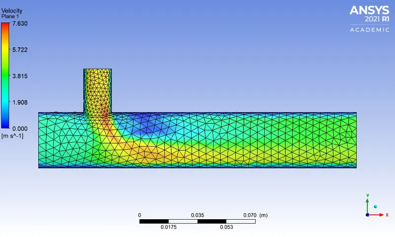
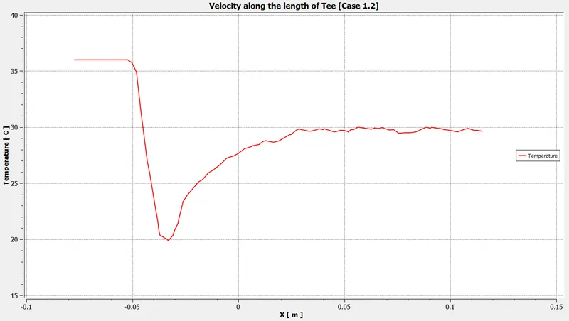
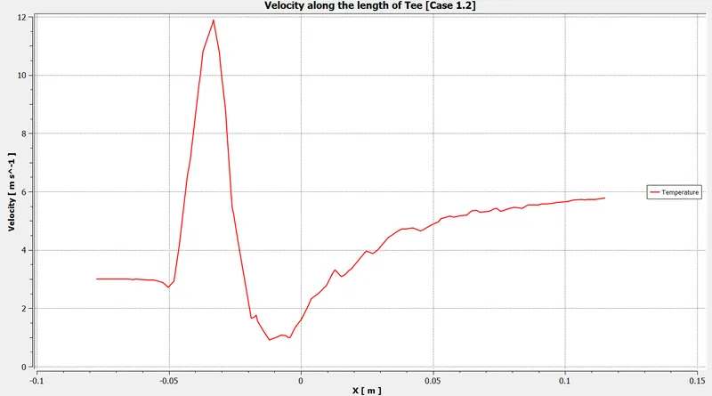
• The 'mixing of the two streams' can be observed from the temperature contours. Due to turbulent mixing, there exists a high-velocity field and a low-pressure field in the region. This point can be observed from the line plots shown below for better clarity.
• Case 1.1 depicts a small diffusion zone that does not affect the temperature at the bottom walls of the Tee. As the momentum ratio is doubled, the diffusion zone further penetrates deep into the hot stream affecting the temperature of the walls below it as observed from case 1.2. The higher momentum ratio increases the effectiveness of mixing as well. The same trend is observed in the longer Tee.
• The temperature contour and the velocity contour indicate that for the short Tee, the hot stream and the cold stream can be seen distinctly at the outflow boundary. But with the longer tee, better mixing is obtained at the end of the Tee and the temperature over the outflow boundary is more uniform.
• A region of low velocity is formed next to the entry of the cold stream. This is due to such geometrical design of the Tee.

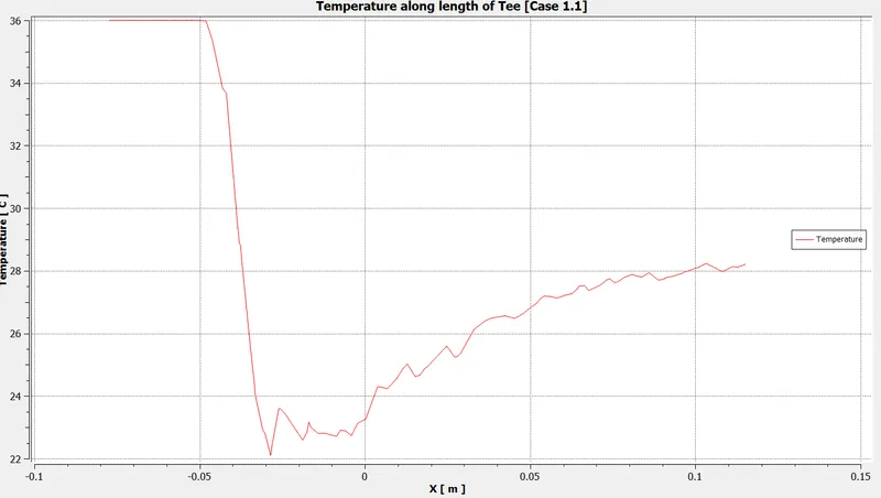
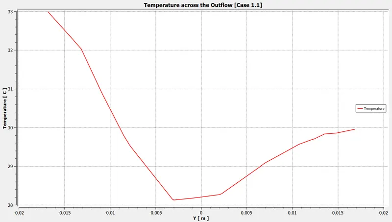
v) Line Plot of temperature along and across the Tee [Case 1.1]

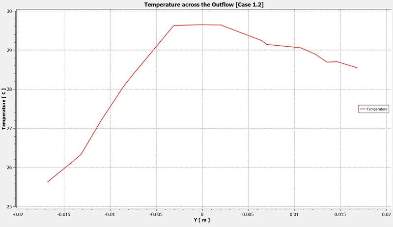
vi) Line Plot of temperature along and across the Tee [Case 1.2]

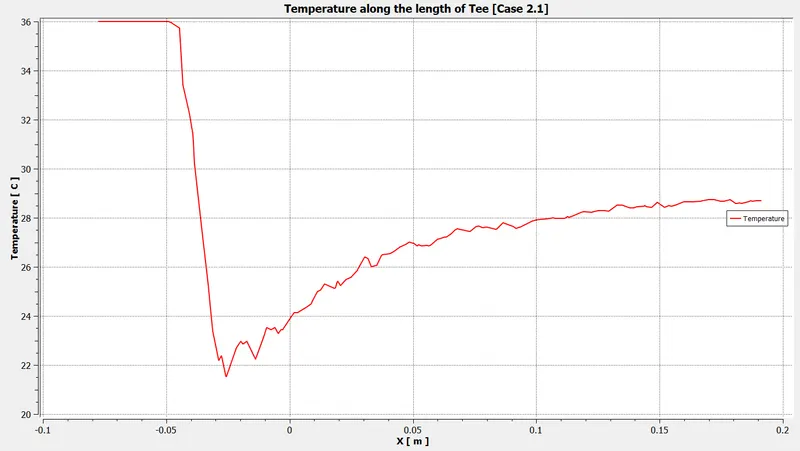
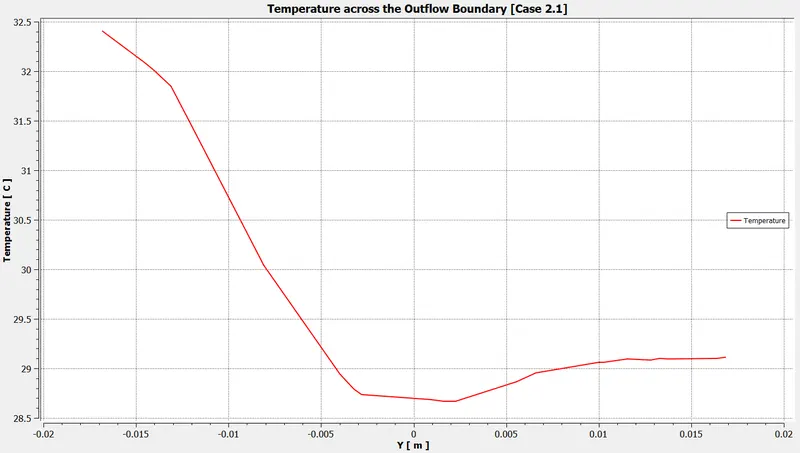
vii) Line Plot of temperature along and across the Tee [Case 2.1]

viii) Line Plot of temperature along and across the Tee [Case 2.2]

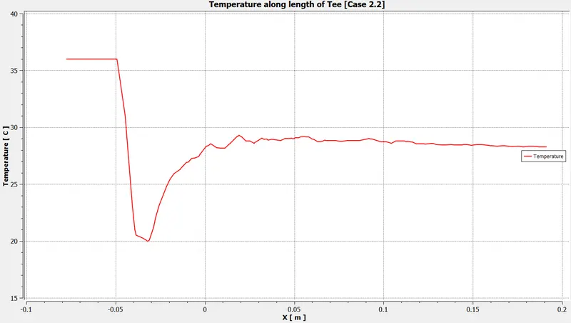
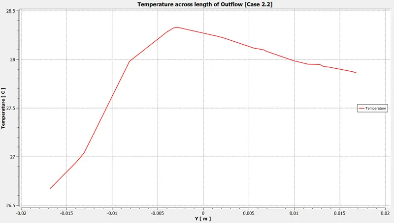
• From the Temperature VS length of Tee plot, a sudden drop in temperature is observed due to the sudden entry of the cold stream from Inlet_Y. The variation of temperature during mixing can be observed from the gradual increase in temperature just after the drop. This increase in the temperature is more erratic in the cases with a smaller momentum ratio. The gain in temperature is more gradual and becomes more predictable with an increase in the momentum ratio.
• From the Temperature VS Y distance plot, in the case 1.1, the temperatures across the cross-section are bound between 28 deg C and 33 deg C. Considering the origin somewhere in between the C/S, the lower wall depicts a temperature value of ~33 deg C because of the undisturbed hot stream that flows along the bottom wall. The temperature drops from 33 and increases across the C/S due to the mixing.
• In case 1.2, the momentum ratio is doubled. The temperatures at the outflow are bound between ~25.5 deg C and ~29.5 deg C implying a lesser standard deviation. The temperature at the lower wall is ~25.5 deg C and the temperature increases to a maximum and drops in contrast to the opposite behavior obtained in case 1.1. The bottom wall no longer contains an undisturbed hot stream but contains a mixed stream of lower temperature which is clear from the temperature contour of the case.
• The same trend is observed in cases 2.1 and 2.2

c) Grid Dependence Study:

The challenge is carried out with a base mesh of 0.005m. In this section, the grid is further refined, and the percentage of error obtained in the solution is calculated. The parameter that is checked for grid independence is the standard deviation of temperature and average outflow temperature. If the parameters converge to a particular value within a marginal range of error with further refinement in the grid size, the problem is said to be grid-independent and the solution obtained is accurate. The grid dependence study is carried out for case 2.2.

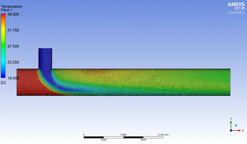
Temperature Contours with increasing refinement:

i) Grid Size 0.005m

ii) Grid Size 0.004m

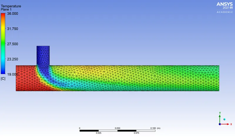
iii) Grid Size 0.002m

The values of standard deviation and average outflow temperature obtained at the outflow are shown below:

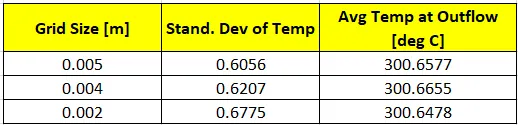
• With refinement in mesh, the average temperature at outflow does not increase significantly and has converged up to two decimal places and the standard deviation of temperature is accurate up to one decimal place.
• The diffusion of temperature is being captured more accurately with further refinements and at the mesh size of 0.002m, the mixing phenomenon is relatively much accurate and can be considered as a grid-independent solution.
• At the base grid of 0.005m, the error in the standard deviation of temperature is 11.87% and the error in the average temperature at outflow is 1.50%

CONCLUSION:

1. Four cases with capturing the mixing of the hot and cold stream, with varying momentum ratio and varying length of Tee is simulated
2. Velocity and temperature contours and line plots are plotted on the cut planes along and across the pipe.
3. Mesh independent study is performed.
4. The effect of length and momentum ratio on the results is discussed.