Simulating Rayleigh Taylor Instability using Fluent

OBJECTIVE:

To simulate the Rayleigh Taylor Instability under two different criteria; One, To observe the instability with mesh refinement; Two, To understand the effect of density of the material used, on the instability.

SOFTWARE USED:

1. Ansys Fluent 2021 R1

RAYLEIGH-TAYLOR INSTABILITY:

The Rayleigh Taylor instability [RTI] is a hydrodynamic instability observed when a dense fluid is present over a low-density fluid in a gravitational field. The RTI is responsible for phenomena as simple as falling of water when the glass of water is inverted to phenomena like the formation of astrophysical objects like supernova remnants. The RTI is an important subject in the study of Multi-phase flows.

General Mathematical Model of RTI:

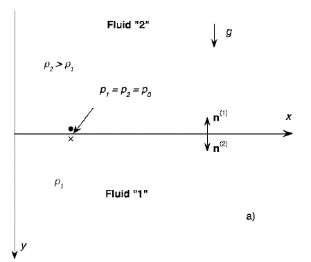
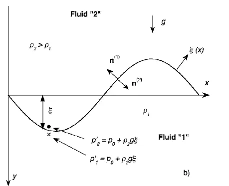
One of the new approaches to model the RTI is using Newton's 2nd Law [1]. According to this model [1], initially, the Interface is assumed to be planar and at equilibrium at a certain pressure `punderset(o)()`. A small perturbation is introduced at the interface such that the elements at the interface us quasi-statically transported to the perturbed wave. It is known that, with depth, the pressure increases linearly. Now, the pressure difference across the perturbated interface is proportional to the densities of the fluids. This pressure difference drives the instability and the motion of the interface. The pressure difference multiplied by the area of the interface gives the net driving force that is equal to mass times the acceleration according to Newton's 2nd Law.

`m ddot zeta = trianglepA` -------------------------------------(A)

It is assumed that the RTI induces surface motion that decays as `exp(-ky)` where `k=(2pi)/lambda` is the wavenumber and `lambda` is the wavelength of perturbation. The mass 'm' is the total mass that moves with the interface and is contained within the distance proportional to `k^(-1)`. With some manipulation, (A) can be written as:

`frac{rhounderset(2)()+rhounderset(1)()}{k}ddotzeta = (rhounderset(2)()-rhounderset(1)())gzeta`

(or) `ddot zeta = Aunderset(T)() kgzeta` --------------------(B)

where `Aunderset(T)()` is the Atwood Number given by `Aunderset(T)() = frac{rhounderset(2)()-rhounderset(1)()}{rhounderset(2)()+rhounderset(1)()}`

Equation (B) represents the final governing equation for this mathematical model which is valid for ideal fluids. The same argument can be extended to real fluids that require an additional force term at the interface such as viscous forces or surface tension forces.

CFD Model based on RTI used in the challenge - VOLUME OF FLUID Model [VOF]:

The Volume of Fluid (VOF) model is a surface tracking method that finds the interface of two or more immiscible liquids. The phases in each cell of the mesh are known by the Volume Fraction of the cell. The equations involved in the VOF modeling are the i) Volume fraction equation, ii) Momentum equation iii) Energy equation.

The volume fraction equation is basically the solution of the continuity equation for each phase and its solution gives the volume fraction of the phase. The sum of volume fraction of all phases in a cell must be equal to 1. Both explicit schemes and implicit schemes are used to solve the volume fraction equation. The transient formulation is used for both steady and transient states. The explicit formulation is used for transient states only. Shown below is the volume fraction equation for a phase 'q'. Here 'p' represents another phase.

The Momentum and the Energy equation are shared by all the phases. The density and viscosity of the phases in a cell influence the resulting velocity.

The Atwood Number:

The Atwood number is a dimensionless number used in the study of hydrodynamic instabilities in density stratified flows. It is a dimensionless ratio of the difference of the densities of the two fluids to the sum of the densities of the two fluids. Atwood number is an important parameter in the study of Rayleigh–Taylor instability. For Atwood numbers close to 0, the RT instability flows take the form of symmetric 'fingers' or 'mushroom clouds' of fluid; For Atwood numbers close to 1, the lighter fluid that is 'below' the heavier fluid takes the form of large bubble-like patterns.

`At = frac{rhounderset(1)()-rhounderset(2)()}{rhounderset(1)()+rhounderset(1)()}` where `rhounderset(1)()` is the density of the heavier fluid and `rhounderset(2)()` is the density of the lighter fluid.

CASE SETUP FOR RAYLEIGH TAYLOR INSTABILITY USING VOF METHOD IN FLUENT:

I) Introduction:

A 2D simulation is performed to understand the instability. The physical model basically contains two domains sharing a single edge. The two domains contain the two phases. The shared edge represents the interface of the two phases. This setup is then run with a transient solver to observe the instability. Three cases are set up in this problem.

1. Case #1 uses a base mesh of 0.5 mm with air and water as the phases.
2. Case #2 uses a refined mesh with air and water as the phases
3. Case #3 uses the same refined mesh with water and a user-defined material as the phases.

The Atwood number in the case of water and air is calculated as 0.9975490.

The Atwood number in the case of water and UDM is calculated as 0.4278359.

II) Geometry:

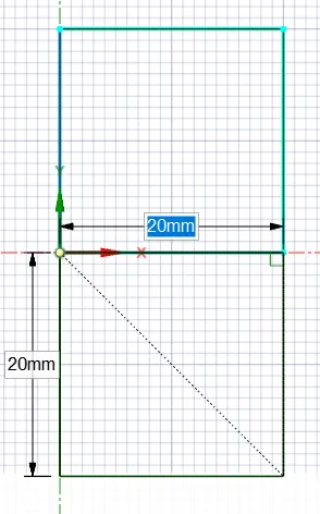
Two 2D domains (square of side 20 mm) with a common edge are created in Spaceclaim to hold the two phases. The two domains are shared using the 'share' option under the Workbench tab in SpaceClaim in order to create a conformal mesh.

III) Meshing:

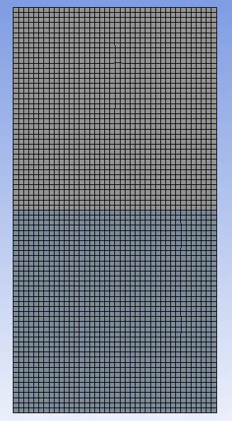
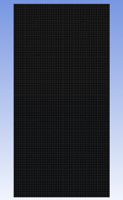
Since the geometry is very simple and consists of straight lines, the default mesh generated is of square type. The base mesh size used for the problem is 0.5 mm. The total cell count, in this case, is 3200. The mesh size used in the refined case is 0.1 mm. The total cell count, in this case, is 80000. Shown below is the base mesh on the LHS and the refined mesh on the RHS. It is known that the RTI is to be simulated under Laminar conditions. Hence, there is no consideration of Y+ and its effect on the mesh.

IV) Fluent:

• A pressure-based, Transient solver is used. The transient solver is chosen to capture the instability at the interface that collapses w.r.t time. Gravity is enabled. The acceleration due to gravity is set to -9.81 m/s^2 in the -Y direction.
• A steady-state VOF simulation makes sense only when there are distinct inlet boundaries for different phases.
• Under viscous models, the Laminar option is chosen, as the flow is essentially laminar.
• From the material library, air and water are chosen. The material properties are constant and do not change. In case #3, the air is replaced by a user-defined material (UDM) with the following properties: Density = 400 kg/m³, Viscosity = 0.001 kg/m-s.
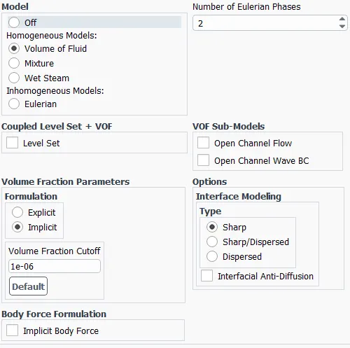
• The multiphase model is clicked and the Volume of Fluid method is chosen. The number of eulerian phases is set to 2. The Implicit formulation is chosen as the problem is a transient one.
• The material of the primary phase (water) and the secondary phase is selected (air). The material can be chosen in the other way round also. In case #3, the air is replaced by UDM.
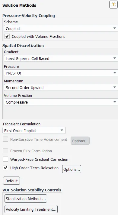
• The solver settings are shown below. The solver scheme is set to 'coupled'. In this scheme, the momentum and species continuity equations are solved together using coupled AMG. The pressure interpolation scheme is set to PRESTO! The PRESTO! (PREssure STaggering Option) scheme uses the discrete continuity balance for a "staggered" control volume about the face to compute the "staggered" (that is, face) pressure. The 'compressive' interface tracking scheme is used for the reconstruction of the face values of VOF at the interface.
• It is necessary to provide the right under relaxation factors to prevent a floating-point error and divergence of the solution. This VOF problem is very sensitive to larger time steps and smaller mesh sizes.
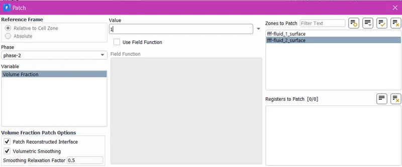
• Next, the solution is initialized. To initialize, the two domains have to be 'patched' with the respective volume fraction of any one phase, say, air(phase-2). The upper domain must contain the denser material and must be patched with water. The lower domain must contain air. This is done by setting the volume fraction of air as 0 in the upper domain and setting the volume fraction of air as 1 in the lower domain.
• In case #3, the density of the UDM is lesser than that of water. Hence volume fraction is patched in such a way that water is present in the upper domain and UDM is present in the lower domain.

• Next, the contour of the volume fraction is set up. Animation of the volume fraction contour is set up.
• Lastly, the time step size is set to 0.005 sec, and the number of timesteps is set to 1500. The case is now run.

RESULTS:

1) Convergence:

Case #1:

Case #2:

Case #3:

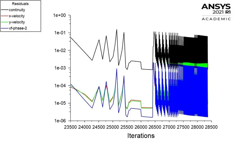
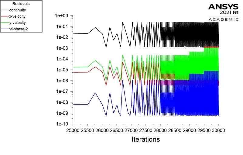
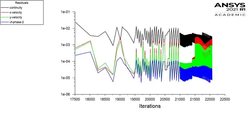
• The residual plot shows the residuals for continuity, velocities, and volume fraction of phase 2. A repeated pattern is observed in the residual plots indicating convergence.
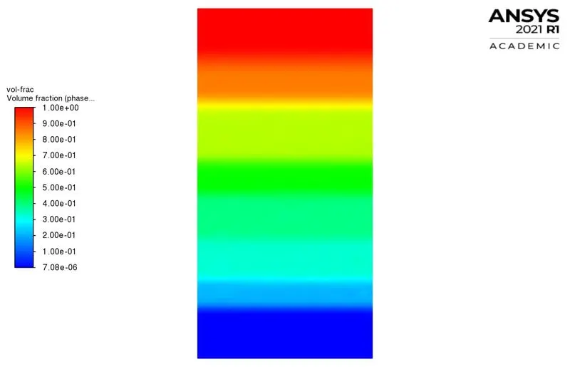
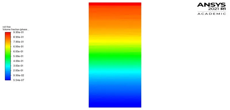
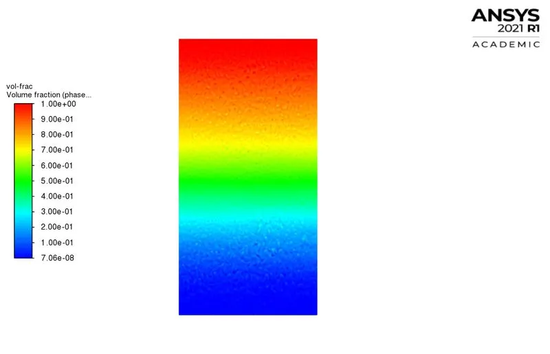
• Also shown is the final volume fraction contour of the respective phase 2. It is observed that the contour did not change significantly wrt time after a few thousand iterations (not shown).
• Hence it can be said that the problem has converged.

2) Contours and animation of Volume fraction of the respective Phase-2:

Case #1:

Case #2:

Case #3:

• Shown above is the final volume fraction plot of phase-2 on the LHS and the variation of the volume fraction contour wrt time on RHS for each case.
• The instability of the interface is observed in the animation. After going through an unstable phase, the heavier fluid settles at the bottom, and the lighter fluid settles on top. The middle of the domain is taken over by cells containing an equal amount of both phases [volune fraction = 0.5]. Bands of other volume fractions can also be observed from the contour.
• The instabilities start off as straight lines and immediately takes the shape of mushroom clouds or finger-like projections with the lighter fluid (air) penetrating into the heavier fluid. This penetration of the lighter fluid into the heavier fluid grows deeper and a series of shapes are patterns are formed. Swirl-like patterns are formed in the flow. They are observed to be single-layered.
• In Case #2, the development of the instability becomes more clear with refinement in the mesh. The Atwood number is close to 1. The swirls that are formed in this Case contain thin layers of the other phase and thin layers of volume fraction of 0.5. The patterns formed are mostly swirling. They diffuse and transport the lighter fluid into the heavy fluid.
• The magnitude of perturbation is observed to be more intense. The sizes of the swirl are much larger. This refined case takes much more time to settle compared to the baseline. Even after settling, small bubble-like formations are observed.
• In Case #3, a user-defined material is defined, the Atwood number decreases (in this case, a denser material compared to air); The density difference between the two fluids is reduced. It is observed that the intensity of instability of the interface is relatively reduced; The swirls are smaller in size, are more in number, and are observed for a longer duration. The bubble-like formation becomes more prominent and is constantly in motion even at the end of the simulation.
• From the theory of RTI [1], it is known that with a decrease in Atwood number, the perturbation intensity is less but its effects linger for a longer duration. With an increase in Atwood number, the driving force of instability increases, and the time for which the swirls and instabilities arriving at the bottom of the domain is reduced.
• This is what is observed from the animations of Case #2 and Case #3.
• Hence the simulations conducted in this challenge are validated.

CONCLUSION:

• The Rayleigh Taylor Instability is carried out using the Volume of Fluid (VOF) technique and a transient solver. The Atwood number is defined.
• The instability is very sensitive wrt the time step and the mesh size. Under relaxation is necessary to prevent divergence of the simulation.
• With refinement in the mesh, the instability patterns are more clear and different bands of volume fractions are observed in the final volume fraction contour.
• With the increase in Atwood number, the intensity of the instability increases, and the time taken for the instability to settle down decreases.

References:

[1]: Study of Rayleigh Taylor Instability with the help of CFD simulation, Indrashis Saha, Department of Chemical Engineering, University of Calcutta, Kolkata, India

[2]: The Rayleigh-Taylor instability, A. R. Piriz, O. D. Cortázar, and J. J. López Cela