Shock tube simulation using CONVERGE

OBJECTIVE:

In this challenge, a transient simulation of flow through a Shocktube is carried out using Converge. The effect of the shockwave is also recorded.

SOFTWARES USED:

1. Converge Studio v3.0
2. Windows CMD and CYGWIN
3. Paraview

A BRIEF INTRODUCTION TO SHOCK TUBE AND A NOTE ON REGIONS AND EVENTS:

Shocktube:

The Shocktube is a tube made out of metal that consists of two chambers separated by a diaphragm. The two chambers consist of two gases with a large pressure ratio. The gas of higher pressure is called the Driver Gas and the other one is called the driven gas. The chambers are also termed Driver and Driven.

The diaphragm is builtin with a puncturing mechanism that breaks the diaphragm under predetermined conditions.

The breaking of the diaphragm causes a drastic onset of compression pressure waves towards the low-pressure region due owing to a sudden pressure difference. The leading pressure wave is called the Shockwave. This shockwave is followed by a series of more pressure waves which raises the temperature and pressure of the driven gas. Simultaneously, a rarefaction wave formed in the opposite direction of the shockwave which travels towards the driver chamber.

One of the main applications of shock tubes includes the study of the chemical kinetics of fuels. The chambers of the shock tube would be filled with an Air-Fuel mixture; As the shock propagates, the pressure and temperature rise. When the temperature attains the auto-ignition temperature, the fuel ignites. Hence this can also be used to find the auto-ignition delay of the fuel.

Regions and Events:

In Converge, a 'Region' is a collection of boundaries used to delineate different areas in a geometry. Let us take the example of the shock tube itself. In the shock tube, there exists a High-pressure(HP) region and a Low-pressure(LP) region. These two must be separated initially which is taken care of by regions.

Events is a feature that engages and disengages two boundaries. In a real shock tube, there is a diaphragm that prevents mixing between the two chambers. To incorporate this effect in the simulation, a region is added, and using events, the disengagement of the region is simulated. At time t>0, the initial engagement is disengaged and the pressure difference creates a shockwave.

Internally, the Converge solver creates a temporary obstruction using triangles to from regions. These temporary triangles are called Disconnect Triangles. There are two types of disconnect triangles- Single Loop and Concentric.

In the shocktube simulation, single-loop disconnect triangles are used, as the interface region between both the regions are of the same dimensions;

CASE SETUP IN CONVERGE STUDIO:

The Geometry is given in form of a .stl file. It is then is imported into Converge.

1) Geometry:

The bounding box of the geometry is of dimensions are 0.2m X 0.01m X 0.01m .

2) Materials:

Gas ==> Air (N2 and O2) selected in species.in

3) Mesh:

The base mesh is of size 0.001m in all three directions.

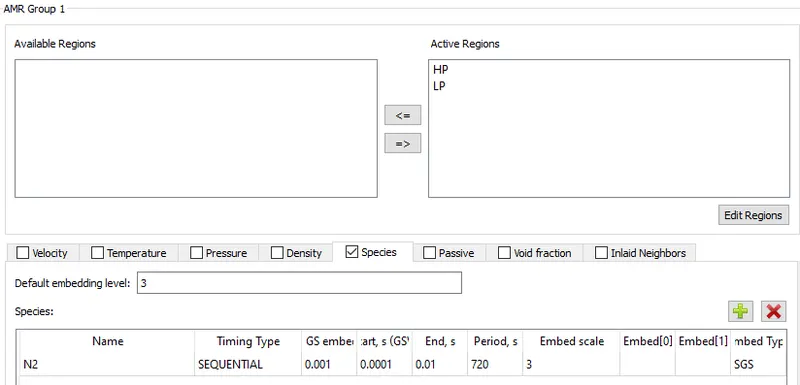
The Adaptive Mesh Refinement (AMR) option is enabled. AMR is applied to species concentration. AMR timing is set to sequential meaning AMR sequence will be executed only once at the selected regions. The embed scale is set as 3. Hence the smallest cell size will be `0.001/(2^3) = 0.000125 m`. The embed type is set to SGS. This means a minimum mass fraction of the selected species (N2) will activate the AMR.

4) Boundary Conditions:

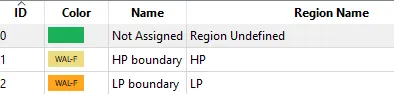
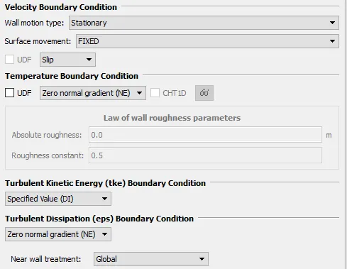
The geometry is flagged into two regions: the complete left side (HP) represented by green color and the complete right side (LP) represented bt brown color. Both the boundaries are 'WALLS' with a slip condition on velocity and 'ZeroNormal' [Neumann] Temperature Gradient.

5) Initial Conditions and Events:

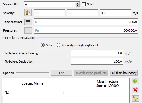
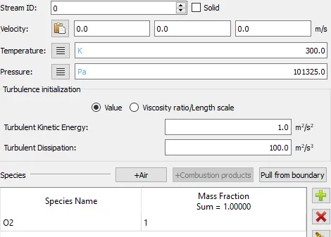
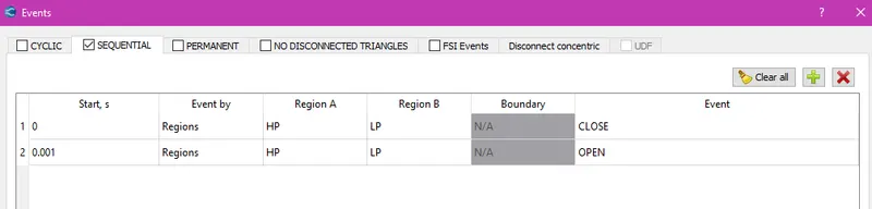
Initially N2 is present at 6 bar at a temperature of 300 K on the HP chamber and O2 is present at 1 atm at a temperature of 300 K on the LP chamber. The two events are initialized sequentially, the first one being HP and LP regions being disconnected/closed @ 0 seconds and second one, HP and LP regions connected/ opened @ 0.001 seconds.

6) Simulation and Time parameters

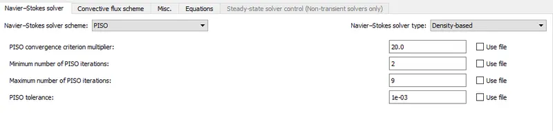
The N-S solver is set to PISO (Pressure Implicit with Splitting of Operators) which is predominantly used to handle unsteady simulations. It uses the concept of pressure correction; The algorithm uses 1 predictor step and 2 corrector steps to arrive at an accurate value for the pressure correction term. The solver type is set to Density-based as the problem deals with high-speed compressible flows.

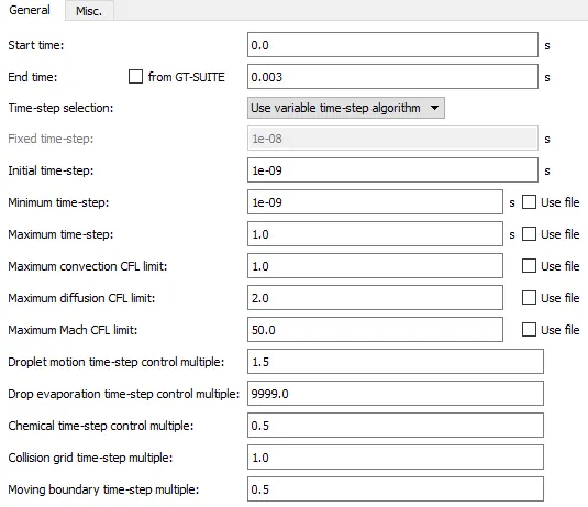
Transient Simulation start time 0 seconds and end time of 0.003 seconds.

7) Turbulence properties:

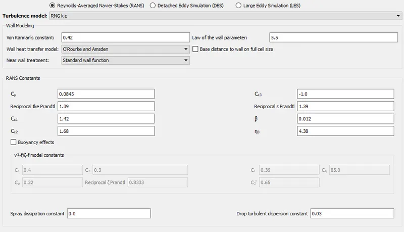
RNG `k-epsilon` turbulence model is set for the case. Generally, the standard `k-omega` SST model is used at the industrial level. Not many differences exist between RNG `k-epsilon` and the `k-omega` SST model.

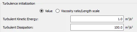
The (Initial Conditions) initial value of Turbulent Kinetic energy 'k' is assigned to the default value of 1 `m^2s^-2` and Turbulence Dissipation rate '`epsilon`' is assigned to the default value of 100 `m^2s^-3`.

The basic idea of the RNG `k-epsilon` model is to solve the transport equations involving Turbulent Kinetic energy 'k' and Turbulence Dissipation Rate '`epsilon`' to arrive at the values of k and `epsilon`. With the values of k and `epsilon`, the Eddy viscosity can be calculated. With the value of Eddy viscosity, the Reynolds stresses, and further, the RANS equation can be solved for average velocity. Shown below are the default RANS constants which are to be used in the k-`epsilon` transport equation.

Output/Post-processing:

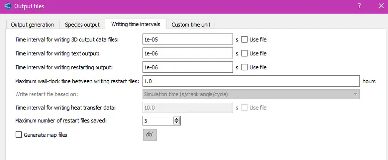
To obtain a smooth animation in post-processing, the intervals at which 3D data is written is set to 1e-5. This creates 300 3D data files. And to enable accuracy in plots, the interval at which text data is written is set to 1e-6. This creates 3000 text data files.

EXPORT OF INPUT FILES:

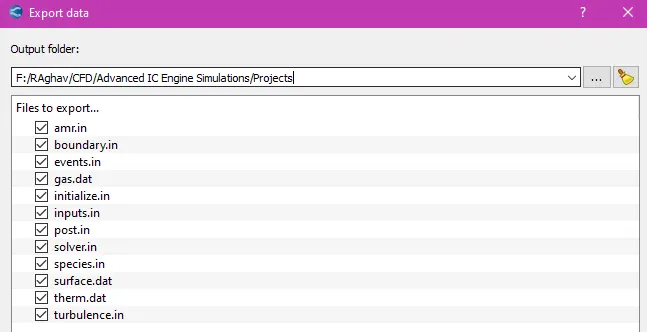
In Converge Studio, the case set-up of the problem is done. This essentially creates all the necessary input files for the Converge solver. Once the case setup is done, the input files are exported to a new folder. Shown below are the input files that have been generated by Converge Studio.

RUNNING THE SIMULATION:

A Command-line editor tool like Windows CMD or CYGWIN is used to set up the run. Here Windows CMD is used. Firstly, the location of the input files is navigated to and the Converge solver is called using the Command Line tool. For faster computational speed, parallel processing is set up on 4 cores using INTEL MPI software.

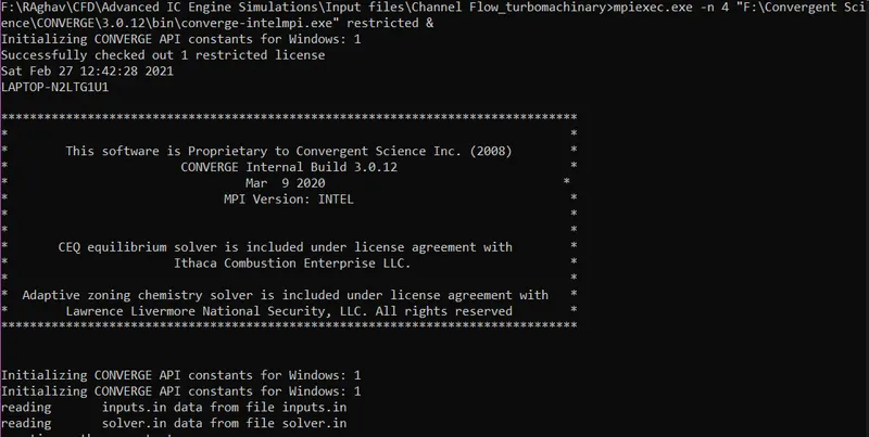
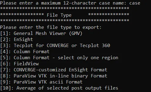
At the end of the run, the solver generates "post.h5" files (3D Output files) and ".OUT files" (Data files). The ".OUT" files contain data at mesh points. The 3D Output files are further post-processed using Converge post-processing tool into "Paraview VTK-Inline Binary format" to further analyze the case in Paraview.

RESULTS & OUTPUT:

A) Mesh:

The first image represents the base mesh of 0.001m. The second image shows the mesh when AMR gets activated. The smallest size of the cells is given by 0.001/(2^3) which is 0.000125m.

B) Temperature Plot and Contour:

• The above plot is obtained at the instant the diaphragm is broken.
• The temperature is initially 300K at both the regions. Once the diaphragm breaks, due the pressure difference, the shockwaves sets in and this causes an increase in temperature in the driven region.
• Towards the left side of the diaphragm (driver region), rarefaction waves are set into motion, which casuses the expansion process, and hence there is a decrease in temperature from the ambient.
• When the shockwave hits the right end, its temperature increases further and gets reflected back. It now travels towards the other end of the tube heating the contents of the tube even at the driver side where the contents are below ambient temperature due to the rarefaction wave.
• Upon getting reflected back, its temperature further increases, and once again it travels towards the right end heating all the contents as it propagates.
• When it hits the right end the second time, the temperature reaches a local maxium and this process keeps repeating.

C) Pressure Plot and Contour:

INFERENCE:

• The image on the left is the pressure plot at t>0 (diaphragm broken). A step in the pressure is formed exactly at the position of the diaphragm and an increasing gradient of pressure is formed in the driven side and decreasing gradient of pressure is formed in the driver side.
• The image below is the plot of velocity of the shock. At t=0, velocity is 0. Once the diaphragm is broken, there is a sudden spike in velocity (~230 m/s) at the centre of the tube. If one looks at the plot of the velocity, there are two distinguishable lines one travelling towards the right (shockfront) and other towards left (wavefront of rarefaction wave). Magnitude of velocity of shockfront > magnitude of velocity of rarefaction wave.

Velocity Plot:

• In the pressure animation, we can see that a shock front that moves towards the right, and there exists a rarefaction wave that moves towards the left.
• The rarefaction wave reduces the pressure field w.r.t. its propagation in the Driver section and the shockwave increases the pressure field w.r.t. its propagation in the Driven section.
• The pressure increases with the propagation of the shockwave because, as it moves with high speed, the gas particles in the way of the wave do not get time to move away and it gets pushed along with the initial wave.
• The shockwave upon hitting the ends of the tube reflects back with high pressure and this repeats everytime the shockfront hits the tube ends.

D) Cell count as a function of time:

INFERENCE:

• As the shockwaves keep reflecting back, there is a gradual increase in the magnitude of the curvature of species concentration of N2.
• It is at the simulation time of ~0.001 seconds, that the curvature value goes past the threshold SGS value and hence we see a drastic increase in the number of cells at this point.
• From this time onwards, as the wave keeps propagating, there are a few stagnation points in the concetration of N2. It is because of these points, we are able to observe the up-down pattern in the total number of cells ranging from ~150,000 to ~200,000.

CONCLUSION:

1. The transient simulation of Shockwave is captured.
2. As the diaphragm is broken, there are two waves set into motion, a shockwave that propagates towards the driven region and a rarefaction wave that propagates towards the driver region. The velocity of the shockwave is greater than velocity of rarefaction wave.
3. The characteristic plots such as Pressure and Temperature is plotted.
4. As the shockwave reflects back, there is an increase in the magnitude of pressure and temperature.
5. After the AMR sets in, there is an up-down effect in the number of cells due to the stagnation of N2 species at certain points in the tube.