FSI Simulation on a Turbocharger using Converge

OBJECTIVE:

In this challenge, a transient FSI simulation of flow through the turbine of a turbocharger is carried out for different pressure ratios using Converge. The interaction of the fluid with the turbine wheel of the turbine is captured.

SOFTWARES USED:

1. Converge Studio v3.0
2. Windows CMD and CYGWIN
3. Paraview

BRIEF WORKING OF A TURBOCHARGER:

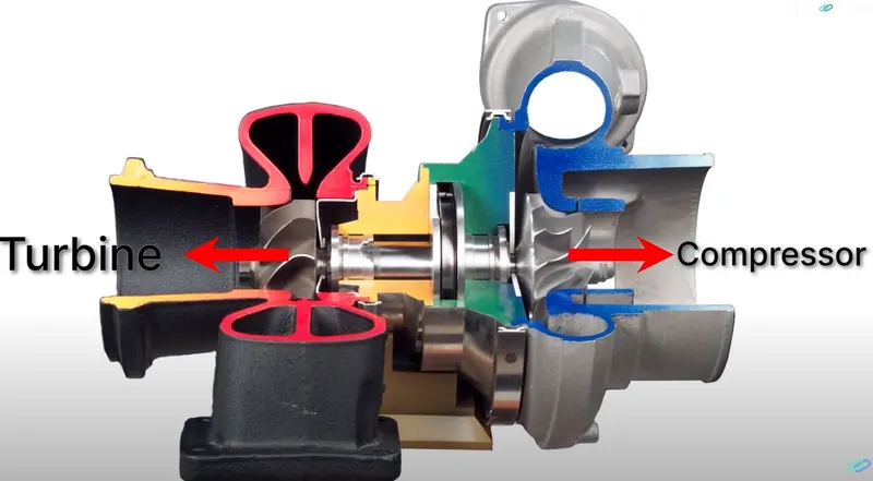
To make an IC engine produce more power, more fuel has to be supplied. To accommodate more fuel, more air has to be supplied for optimal combustion. To increase the amount of air entering the engine, the air is pressurized before sending it to the engine. A Turbocharger is a device that consists of a turbine and a compressor connected by a common shaft. It can be thought of a supercharger (compressor) which is run by a turbine. The assembly as a whole (turbine and compressor) is called a turbocharger.

The work required for the turbocharger is taken from the hot exhaust air of the engine which is rich in enthalpy. This hot air is redirected to the turbine wheel of the turbocharger at a high velocity. This rotates the turbine wheel which in turn rotates the compressor shaft at high speeds. The compressor then compresses the fresh inlet air before sending it to the cylinder.

The main disadvantage of a turbocharger is that it becomes effective only at higher engine speeds. There is also a time lag between the increase in the speed of the engine and an increase in the speed of the turbine wheel. This is called Turbo Lag.

In this challenge, the fluid-structure interaction between the hot air and the turbine wheel is captured. The RPM of the turbine wheel and the Torque required to run the wheel to a pseudo steady state is determined.

Reading a turbocharger map:

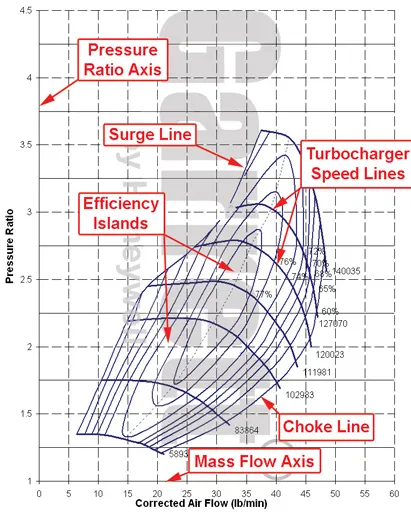
In this challenge, a made-up turbocharger is used. Since the flow is controlling the motion of the turbine wheel, the end time of the simulation is not known. So, a turbocharger map for automotive applications is used to arrive at the simulation end time. The turbo map has 4 quantities: Pressure ratio, Mass flow rate, Efficiency, and RPM. Assuming the operating point to be at a particular efficiency region for a given mass flow rate, the RPM and the pressure ratio can be roughly estimated. Shown below is a general compressor map for automotive applications that is used as a reference in this challenge.

CASE SETUP IN CONVERGE STUDIO:

1) Geometry and flagging:

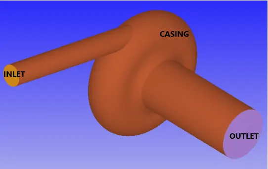
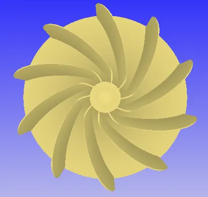
The model of the turbocharger is a made-up geometry since turbochargers are complex models and a CAD model of a real turbocharger is seldom available to the outside market. This challenge is a qualitative one that focuses on capturing the physics of the fluid-structure interaction. The bounding box of the geometry is of dimensions: 0.1727m X 0.0894 m X 0.1114 m

2) Mesh:

The base mesh sizes used are 0.002m in all three directions.

3) Material:

Gas ==> Air

Ideally, the fluid entering the turbocharger must be the exhaust gases. But in this challenge, the main focus is a qualitative study of how the fluid is interacting with the turbine wheel. Hence air is considered for simplicity.

4) Boundary Conditions:

Inlet: Air at a total pressure of 2.5 bar and a temperature of 800K. The case is run for three different pressure ratios: 2, 2.5, and 3. Hence the inlet pressures in cases 1 and 3 will be 2 bar and 3 bar respectively.

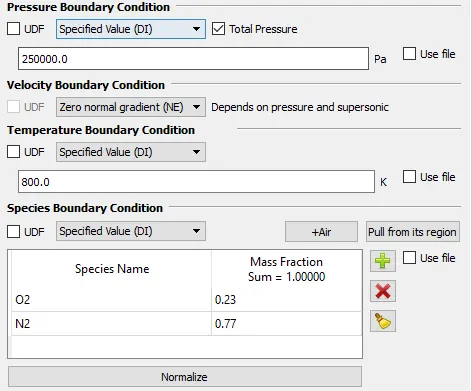
Outlet: The pressure at the outlet is fixed at a value of 1 bar to get the total pressure ratios of 2, 2.5, 3. In the case of backflow, the backflow species is air at 300K.

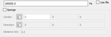
Casing: The casing is specified as a wall with the Law of Wall boundary condition at a temperature of 450K.

Turbine wheel: The turbine wheel is specified as a wall with wall motion type set to FSI.

5) Initial Conditions:

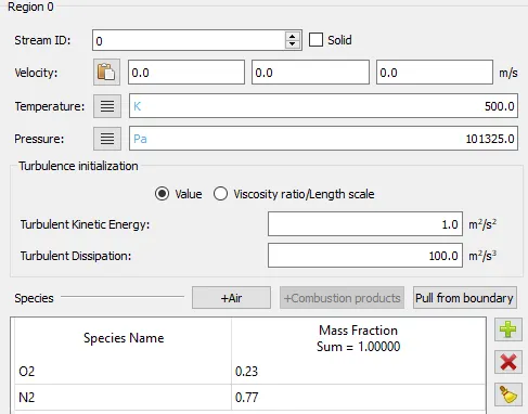
Air at 500K and 101325 Pa.

6) Simulation and Time parameters:

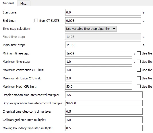
The simulation to be carried out is a gas simulation. The gas flow solver is set to compressible. A full hydrodynamic simulation is performed with a transient solver. The N-S solver is set to PISO (Pressure Implicit with Splitting of Operators) which is predominantly used to handle unsteady simulations. It uses the concept of pressure correction; The algorithm uses 1 predictor step and 2 corrector steps to arrive at an accurate value for the pressure correction term. A density-based solver is chosen to deal with high-speed flows.

End Time Calculation: [With reference to the turbomap]

Corresponding to a pressure ratio of 2.5 (the average of the pressure array used in this challenge) and an efficiency of 77%, the corresponding turbo RPM is ~111985. A value of 100000 RPM is considered in this challenge.

100000 rotations per minute

i.e. 1666.66 rotations per second

i.e. 1666.66 rotations ==> 1 sec

`implies` 10 rotations = 0.006 sec.

Considering the end time of the simulation as 0.006 sec will be a good starting point for a qualitative analysis.

7) Fluid-Structure Interaction (FSI) Setup:

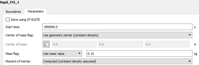
Under the physical models of the case setup, the FSI is enabled. In the FSI setup, a Rigid FSI is selected firstly. Rigid FSI objects can be translated and rotated by pressure and viscous forces, but cannot change shape. When a rigid FSI object is created, the object via fields and options in the Parameters tab must be configured.

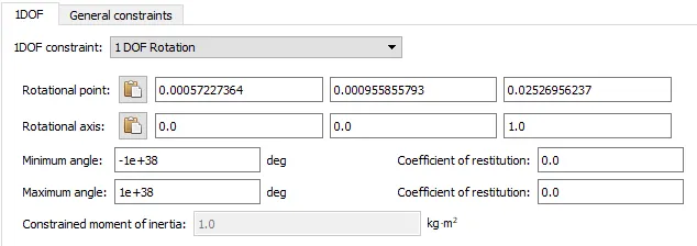
The 'turbine wheel' is selected in boundaries and the parameters such as the mass value of the turbine wheel and its degree of freedom are specified under the parameters tab.

8) Turbulence properties:

RNG `k-epsilon` turbulence model is set for the case. Generally, the standard `k-omega` SST model is suitable for capturing pressure drop. If details such as drag on impeller blades are to be captured, the `k-omega` SST turbulence model would be more suitable.

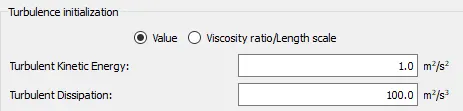
The (Initial Conditions) initial value of Turbulent Kinetic energy 'a' is assigned to the default value of 1 `m^2s^-2` and Turbulence Dissipation rate '`epsilon`' is assigned to the default value of 100 `m^2s^-3`.

9) Output/ Post processsing variables reqd:

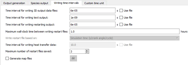
The post-run data variables selected are Pressure, Temperature, Velocity, and Density, Dissipation Rate (`epsilon`), Turbulent KE (k), Turbulent viscosity. The time interval of writing 3D Output files and text files are set such that 100 data files of each are generated. The time interval for restart files is the same as that of 3D output.

EXPORT OF INPUT FILES:

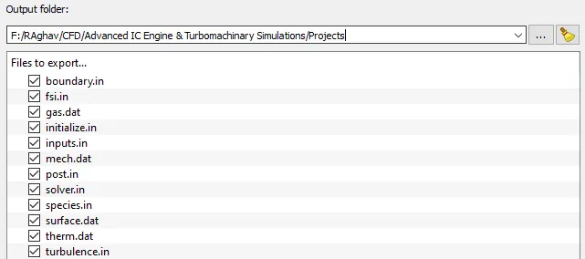
In Converge Studio, the case set-up of the problem is done. This essentially creates all the necessary input files for the Converge solver. Once the case setup is done, the input files are exported to a new folder. Shown below is the list of input files that have been generated by Converge Studio.

RUNNING THE SIMULATION:

A Command-line editor tool like Windows CMD or CYGWIN is used to set up the run. Here Windows CMD is used. Firstly, the location of the input files is navigated to and the Converge solver is called using the Command Line tool. For faster computational speed, parallel processing is set up on multiple cores using INTEL MPI software.

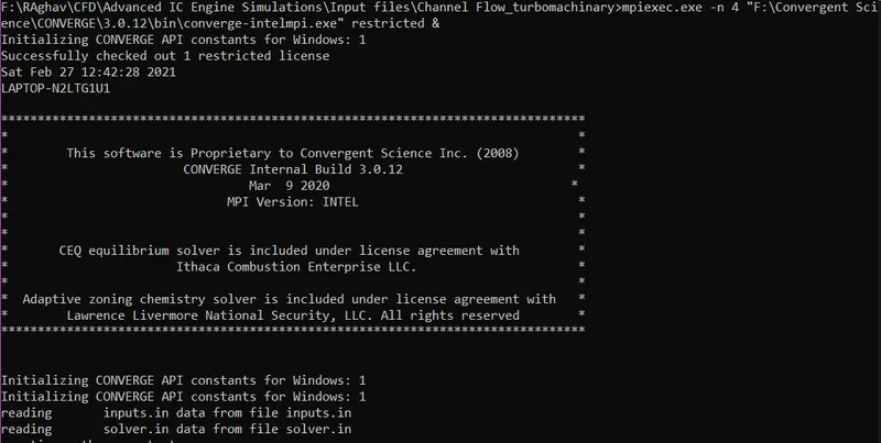
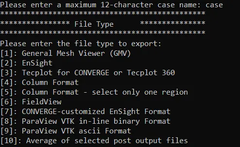
At the end of the run, the solver generates "post.h5" files (3D Output files) and ".OUT files" (Data files). The ".OUT" files contain data at mesh points. The 3D Output files are further post-processed using Converge post-processing tool into "Paraview VTK-Inline Binary format" to further analyze the case in Paraview.

RESULTS:

1) Mesh:

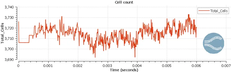
With a base grid of 2mm, the number of cells generated is shown as a function of time.

2) Convergence Check:

Since this is an FSI simulation with a small simulation time, it cannot be said whether the system has attained convergence. Various parameters such as the Mass flow rate, the angular velocity of the turbine wheel, the moment on the surface of the turbine wheel are studied for the test case of 2.5 pressure ratio.

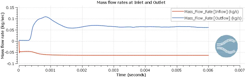
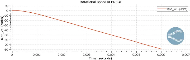
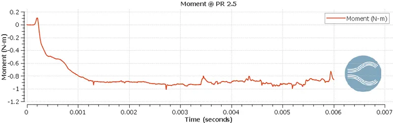
• From the plots, it is clear that the mass flow rate has converged, but the same cannot be said for the other two plots.
• The moment plot (derived from angular acceleration) is fluctuating between a value of 1 N-m and 0.8 N-m. However, it can be said that the moment has attained a pseudo-steady state with respect to an estimation of the 'starting moment' needed to overcome the inertia of the turbine wheel and start motion. It is safe to say that at a time of 0.006 sec, the turbine wheel is already in motion and the initial moment required for motion is ~0.9 N-m.
• From the rotational velocity plot, it is clear that the turbine wheel is still in the accelerating phase and the velocity has not converged.

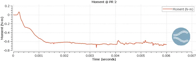
3) Plotting the Rotational speed of the Turbine wheel for different Pressure ratios:

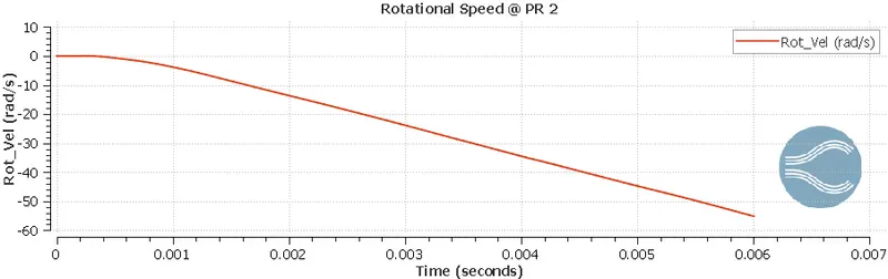
The rotation speed vs time plot is obtained for different pressure ratios from the fsi_object_rigid_fsi.out file.

A) Pressure Ratio 2.0:

B) Pressure Ratio 2.5:

B) Pressure Ratio 3.0:

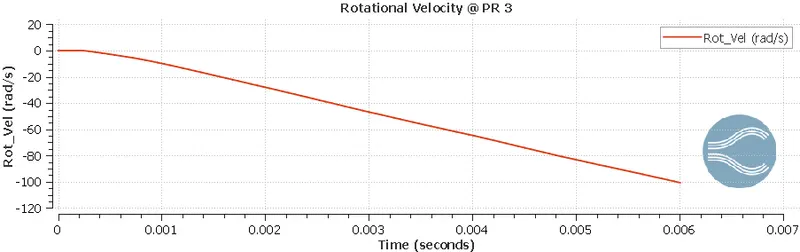
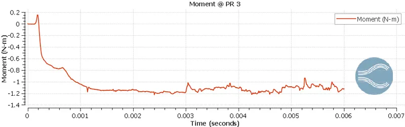
The following table is come up from the plots shown above.

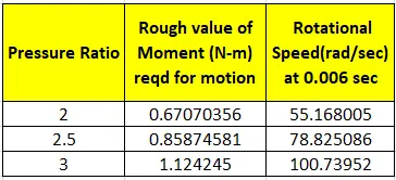
From the table, it can be observed that,

• The moment needed to start motion increases with an increase in the pressure ratio.
• The value of rotational speed obtained at 0.006 sec is higher at higher pressure ratios.

4) Animation Contour of the Pressure and Velocity at a Pressure ratio of 3:

• The FSI interaction is clearly captured from the velocity contour. The blade which is at rest initially starts to rotate owing to the energy transfer. The velocity of the flow decreases in the direction of flow.
• The main drawback of the challenge is that the simulation is performed for a small end time due to limited computational time and resources.
• The pressure contour indicates that there is a formation of a recirculation zone just behind the blade tip. Qualitatively, it can be said that the velocity triangle at the inlet to the turbine blade may be adjusted to extract more energy from the incoming fluid.

5) Calculation of Simulation end time in the case where the Turbine wheel attains its max (or) steady-state speed:

The typical speed of an automotive turbocharger is ~150,000 RPM. With the results that have been obtained, a qualitative estimation of the real run time that is required for the wheel to attain its max speed is made.

For a pressure ratio of 2.5 across the turbocharger, the RPM obtained in this simulation is ~80 rad/sec i.e 764 RPM.

i.e. 764 rotations per second ==> 0.006 sec

i.e. 150,000 rotations per second ==> 1.178 sec

Hence a simulation time of ~1.3 to ~1.4 seconds would be sufficient for the turbine wheel to reach its design speed.

CONCLUSION:

An FSI simulation on a turbocharger is performed and the results are studied qualitatively. The rotational velocity and moment on the turbine wheel at a time of 0.006 seconds is obtained for different values of pressure ratios across the turbocharger. The qualitative prediction of the simulation end time required for the turbocharger to attain its max speed is made.