Supercharger Simulation using Converge

OBJECTIVE:

In this challenge, a transient simulation of flow through a supercharger is carried out for different mass flow rates using Converge. A plot between the total pressure ratio and the mass flow rate is generated.

SOFTWARES USED:

1. Converge Studio v3.0
2. Windows CMD and CYGWIN
3. Paraview

BRIEF WORKING OF A SUPERCHARGER:

For an IC engine to produce more power more fuel has to be supplied. To accommodate more fuel, more air has to be supplied for optimal combustion. To increase the amount of air entering the engine, the air is pressurized before sending it to the engine. A Supercharger is a device that compresses the air before sending it to the engine and it runs on the power supplied from the engine via a connection from the crankshaft. Superchargers are effective at all engine speeds. Superchargers can be positive displacement machines or dynamic machines.

The given supercharger is a Root's type supercharger. It is a positive displacement device. Positive displacement machines are not turbomachines as the pressure rise along a streamline is not due to rotodynamics. A chunk of fluid is taken into space by a rotor and then physically moved/displaced by the rotor from the inlet to the outlet. During this displacement, the volume occupied by the fluid decreases thereby compressing it.

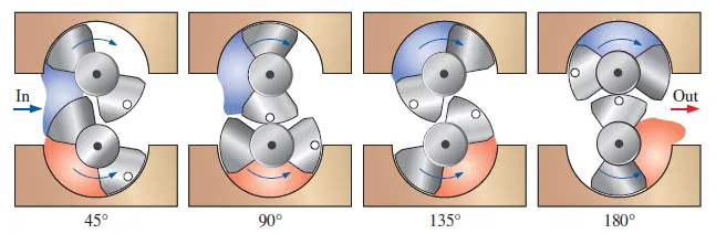
One lobe is powered by a motor. The other lobe is synchronized using an external gearbox. Both lobes rotate in the opposite direction. The pressure at the outlet is controlled by controlling the input power to the machine. The discharge at the outlet is controlled by adjusting the RPM of the motor. One of the disadvantages of a positive displacement device, in general, is that they provide pulsating flow due to the design.

CASE SETUP IN CONVERGE STUDIO:

1) Geometry and flagging:

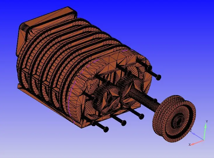
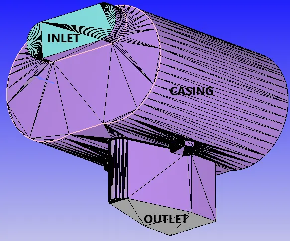
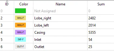
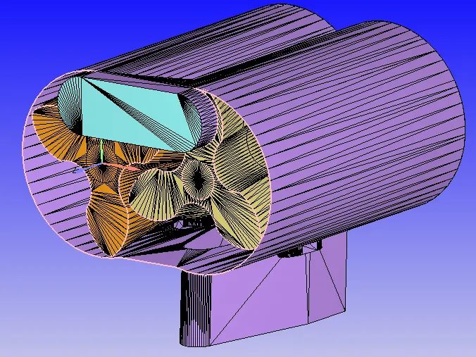
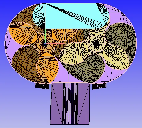
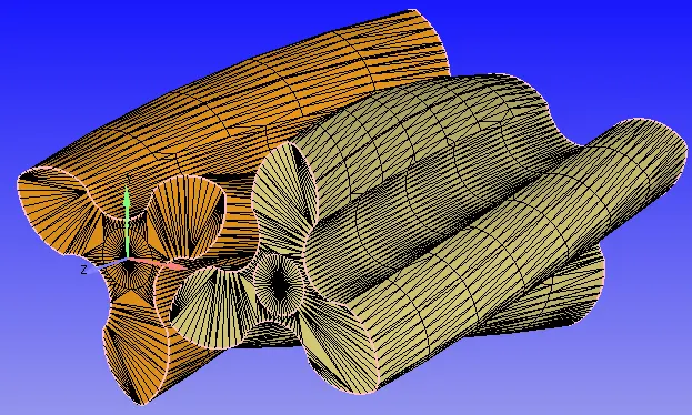
The given Geometry is a .stl file. It is imported into Converge. The fluid domain is extracted from the geometry first. Then , the domain geometry clean-up and boundary flagging are carried out initially. The bounding box of the fluid domain is of dimensions 0.1550m X 0.1430m X 0.1710m

2) Mesh:

The base mesh sizes used are 0.002m in all three directions.

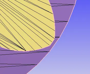
The minimum gap in the geometry must be determined to set up the mesh embedding in that location. This minimum gap is possibly either the one between the lobes and the casing or the one between the two lobes during the rotation. The first case is considered in this challenge as the main motive behind the challenge is qualitative demonstration. At least one cell must be present in the small gap to capture the velocity and pressure gradients accurately. A permanent embed of scale 2 is set at the lobes. Along with this, a velocity AMR is set up to capture the velocity gradients accurately.

3) Material:

Gas ==> Air

4) Boundary Conditions:

Inlet: Air at a total pressure of 1 bar and a temperature of 300K.

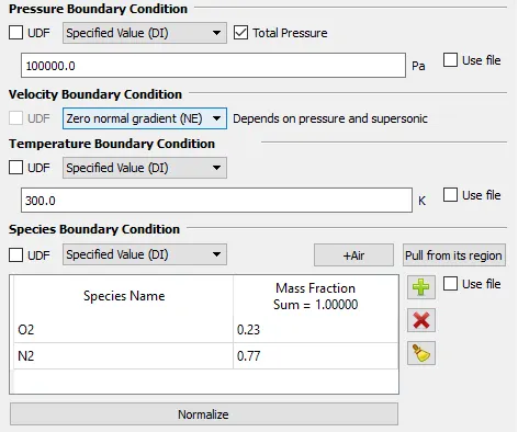
Outlet: The pressure at the outlet is varied to get the total pressure ratios of 1.1, 1.5, 2, 2.2. In the case of backflow, the backflow species is air at 300K.

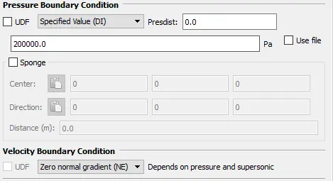
Casing: The casing is specified as a wall with the Law of Wall boundary condition.

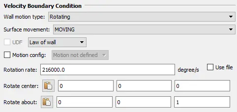
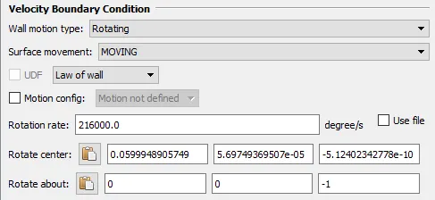
Lobe_left and Lobe_right: The lobes are specified as Rotating walls at a rate of 216000 deg/sec (36000 RPM given) with the Law of the wall boundary condition.

The rotation center of the left lobe is the origin itself. This is done by moving the geometry to the origin with the left lobe's face resting on the X-Y plane. The rotation axis of the left lobe is set to the +Z axis. This will yield a rotation of the left lobe in the anti-clockwise direction. The rotation center of the right lobe is determined by measuring the relative distance between the origin and the center of the right lobe in the X-Y plane. This value is taken as the center of rotation of the right lobe. Its axis of rotation is set to -Z axis. Hence the right lobe will rotate in the clockwise direction. From the image shown below, it can be understood that as the air enters the casing axially, the lobes direct the air around the walls of the casing and stacks it at the bottom of the casing thereby pressurizing it. The air exits radially to the lobes.

5) Initial Conditions:

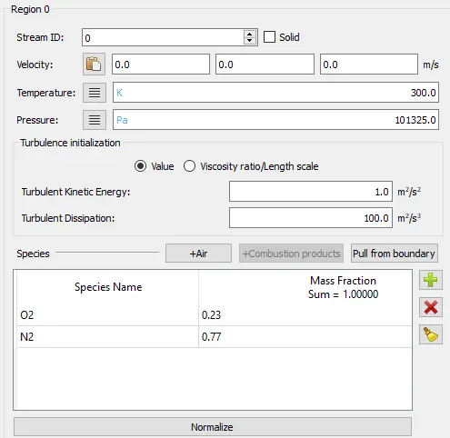
Air at 300K and 101325 Pa.

6) Simulation and Time parameters:

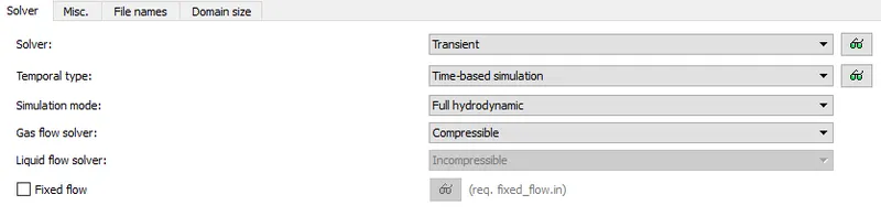
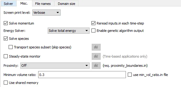
The simulation to be carried out is a gas simulation. The compressor deals with hot air and hence the gas flow solver is set to compressible. A full hydrodynamic simulation is performed with a transient solver. The N-S solver is set to PISO (Pressure Implicit with Splitting of Operators) which is predominantly used to handle unsteady simulations. It uses the concept of pressure correction; The algorithm uses 1 predictor step and 2 corrector steps to arrive at an accurate value for the pressure correction term. Density-based solver is chosen to deal with high-speed flows.

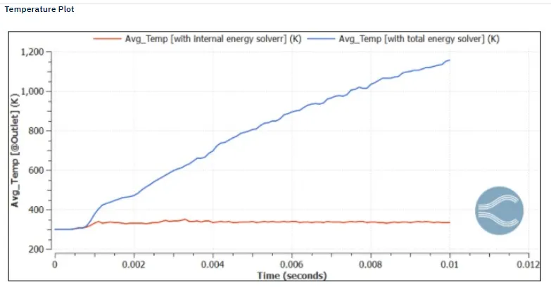
Typically in superchargers, the RPM tends to be very high and the flow attains large velocities. Hence to ensure mass conservation holds at large values of velocity, the energy solver is set to 'solve total energy'. This takes into consideration the internal energy whose change directly affects the velocity from the energy equation.

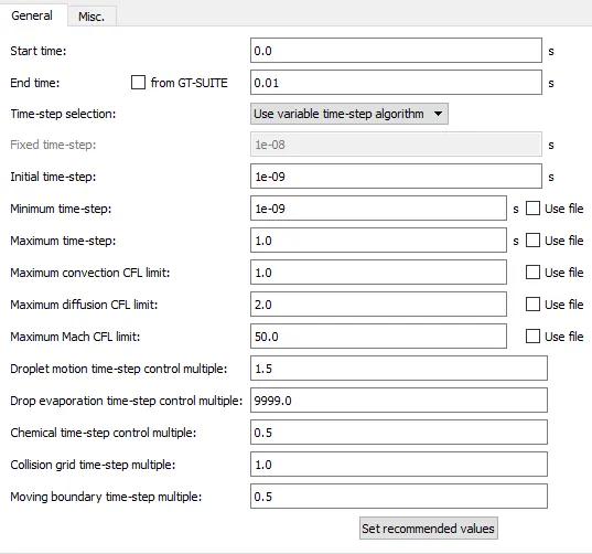
The time parameters are shown below: Simulation start time is 0 sec and end time is 0.01 sec. The impeller must rotate 2-6 times to reach a steady or pseudo steady state.

End Time Calculation:

36000 rotations per minute

i.e. 600 rotations per second

i.e. 600 rotations ==> 1 sec

`implies` 6 rotations = 0.01 sec

7) Turbulence properties:

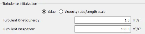
RNG `k-epsilon` turbulence model is set for the case. Generally, the standard `k-omega` SST model is suitable for capturing pressure drop. If details such as drag on impeller blades are to be captured, the `k-omega` SST turbulence model would be more suitable.

The (Initial Conditions) initial value of Turbulent Kinetic energy 'a' is assigned to the default value of 1 `m^2s^-2` and Turbulence Dissipation rate '`epsilon`' is assigned to the default value of 100 `m^2s^-3`.

8) Output/ Post processsing:

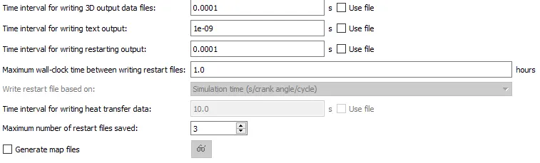
The post-run data variables selected are Pressure, Temperature, Velocity, and Density, Dissipation Rate (`epsilon`), Turbulent KE (k), Turbulent viscosity. The time interval of writing 3D Output files and text files are set such that 100 data files of each are generated. The time interval for restart files is the same as that of 3D output.

EXPORT OF INPUT FILES:

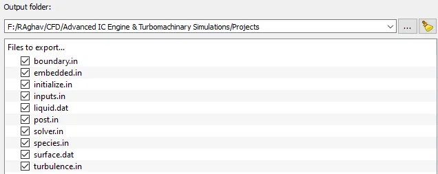
In Converge Studio, the case set-up of the problem is done. This essentially creates all the necessary input files for the Converge solver. Once the case setup is done, the input files are exported to a new folder. Shown below is the list of input files that have been generated by Converge Studio.

RUNNING THE SIMULATION:

A Command-line editor tool like Windows CMD or CYGWIN is used to set up the run. Here Windows CMD is used. Firstly, the location of the input files is navigated to and the Converge solver is called using the Command Line tool. For faster computational speed, parallel processing is set up on multiple cores using INTEL MPI software.

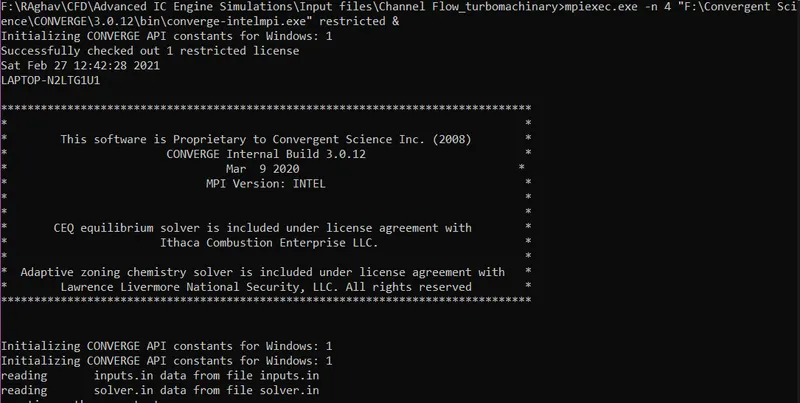
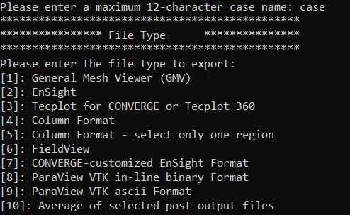
At the end of the run, the solver generates "post.h5" files (3D Output files) and ".OUT files" (Data files). The ".OUT" files contain data at mesh points. The 3D Output files are further post-processed using Converge post-processing tool into "Paraview VTK-Inline Binary format" to further analyze the case in Paraview.

RESULTS:

1) Mesh:

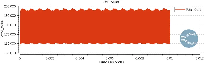
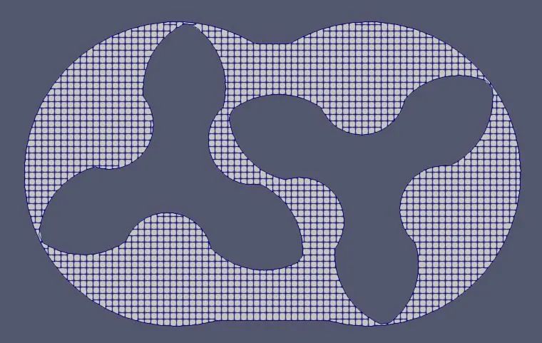
A no-hydro simulation is performed with the specified base mesh, mesh embedding, and AMR. This mode of simulation ignores the transport equations to greatly reduce the computational time and is an efficient way to check for errors in the surface motion and mesh creation. The max cell count is ~198,000.

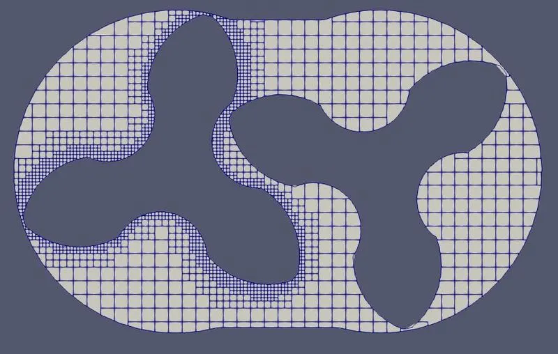
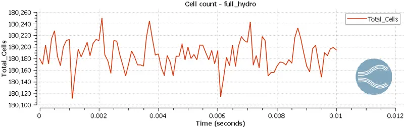
The full hydro simulation is carried out with a relatively finer base mesh but without AMR and embedding keeping in mind the computational time and resources available.

2) Mass Flow Conservation check:

One way to find whether or not convergence has been attained by the simulation is by checking the inflow and outflow mass flow rate values. At steady-state or pseudo-steady state, the mass conservation must hold. For the 4 simulated cases, the MFR check is done.

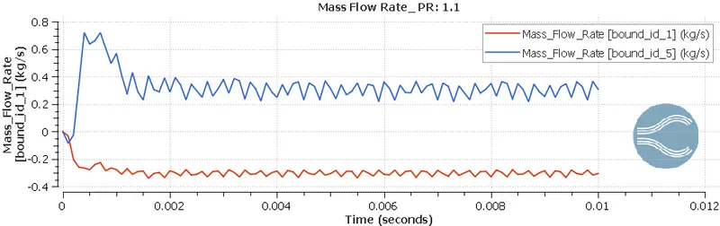
The data of MFR at inflow and outflow at a particular timestep is imported in MS EXCEL for all 4 cases of pressure ratios. The values of inflow MFR and outflow MFR are added. The resulting value after adding should be ideally zero for mass to be conserved but it will not be exactly zero. The allowed difference should not be more than 2e-4 kg/sec.

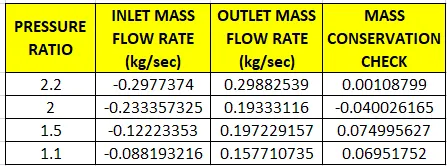
From the tabulated results, it is observed that the differences are greater than the tolerance limit. This can be attributed to two main reasons:

• The fact that the simulation will reach a steady-state or pseudo-steady state with 5-6 rotations of the lobes may not hold in all cases; The simulation may need to run for a longer time.
• The mesh size used is not fine enough and hence yields such values of MFR

3) Effect of Total Energy Solver on the outcome:

Usually, when the energy equation is solved, the internal energy term outweighs the contribution from velocity. This is true for low-speed flows. But in this case, we have high-speed flows and the contribution of the velocity is relatively higher. Hence we solve for total energy. In this simulation, the lobes impart high velocity to the fluid. This velocity change imparts a change in the enthalpy (directly affecting temperature) of the fluid. This work interaction is captured by the total energy solver. This temperature rise due to the work interaction can be seen in the plot shown below.

4) Plotting the MFR vs Total Pressure Ratio Curve:

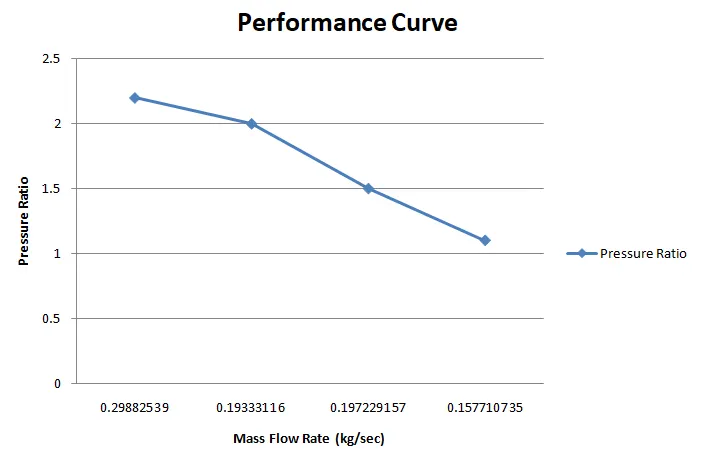
The performance plot is obtained by plotting the Total Pressure ratio VS Mass Flow Rate of the supercharger. The given pressure ratios are 1.1, 1.5, 2, 2.2 for which the mass flow rate at the outlet boundary is obtained from mass_avg_flow.out. The displacement volume of the lobe-type screws is fixed. With increasing mass between the lobes, the max pressure by which the air is compressed must decrease. This trend is captured.

5) Velocity and Pressure Plots & Contours for Pressure Ratio of 1.1:

INFERENCES FROM THE PLOTS AND CONTOURS:

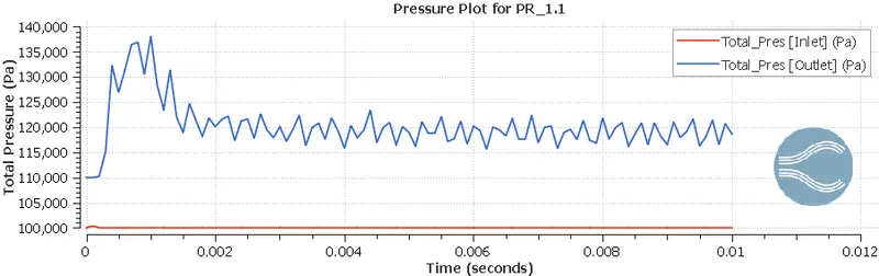
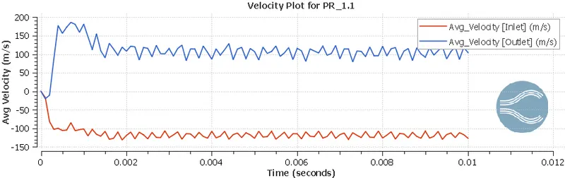
• The pressure and velocity plots have converged.
• Similar trends for velocity and pressure are obtained for all cases of pressure ratios.
• The velocity is higher at the outlet, this is compensated by a decrease in the density to maintain the mass flow rate.
• The mechanism of compression is clear from the pressure contour. The air is transported by the lobes and the rotation of lobes is such that the air gets pressurized close to the outlet after which it is dumped.
• The velocity of flow is maximum just before and after the meshing of the lobes. The velocity of flow leaving the compressor is higher than that of entry.

OUTCOMES FROM THE CHALLENGE:

1. A no hydro simulation with a coarse base mesh is run to ensure that the surface motion is captured correctly. A transient full hydro simulation is then carried out with a relatively finer base mesh. The max cell count is ~180,200.
2. The mass flow rate check is performed to ensure the simulation has reached convergence.
3. In cases of high-speed compressible flows, it is recommended to turn on the total_energy_solver in an effort to capture the work interaction between the fluid and the mechanical component.
4. The performance curve is plotted between the total pressure ratio and the mass flow rate. The trend captured qualitatively in accordance with that of positive displacement machines.
5. The velocity and pressure curves and contours were plotted.
6. The working of the supercharger is simulated and a qualitative study is done.

References:

Fluid Mechanics Fundamentals and Applications by Yunus Çengel, John M. Cimbala