Proportional Safety Relief Valve simulation using Converge

OBJECTIVE:

In this challenge, a CFD study on a safety relief valve is carried out using Converge. The challenge is a two-part study, the first part being, a steady-state simulation to determine the max pressure corresponding to a given lift and the second part is a transient FSI simulation that is to be carried out in order to investigate the dynamic behavior of the relief valve w.r.t. a variable pressure against a constant resisting spring force.

SOFTWARES USED:

1. Converge Studio v3.0
2. Windows CMD and CYGWIN
3. Paraview

Reference:

[1]: CFD simulation of a safety relief valve for improvement of a one-dimensional valve model in RELAP5, ANNA BUDZISZEWSKI, LOUISE THOREN

SAFETY RELIEF VALVE:

A safety relief valve is a pneumatic/hydraulic component that is used to divert the flow from the system to keep the system pressure within the maximum pressure capacity of the system. They are used in every hydraulic or pneumatic line system for safety purposes.

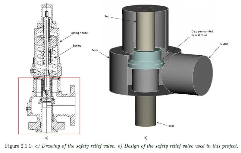
The components and design of the relief valve are shown below. The inlet and the outlet of the valve are at right angles. The valve has a disc that sits on seats (assembly called spindle) blocking the incoming fluid, at pressures lower than the relief pressure setting. A Spring is present above the spindle that exerts a downward force on the spindle providing resistance against the fluid pressure. The relief pressure is set on the relief valve by adjusting the spring tension. The cut section and the 3D model (only the fluid volume, marked in red) of the relief valve are shown below.

The challenge is a two-part study. The first one being a steady-state simulation of the valve to determine the pressure force on the spindle at different valve lifts. The second study aims at investigating the dynamic action of the valve at variable inlet pressure against a constant spring force. An FSI simulation is performed to obtain the results in the second case.

RELIEF VALVE MODELLING:

The steady-state simulation is set up assuming no forces acting on the spindle. The lift of the spindle is adjusted manually and the simulation is carried out. A total of six steady-state simulations are carried out for various lifts: 3mm, 4mm, 5mm. Each case is run with and without Adaptive Mesh Refinement (AMR) and the pressure force is calculated and compared. A steady-state monitor is enabled in these cases.

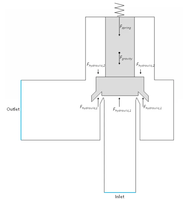
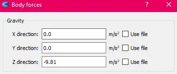
The transient simulation is carried out by considering the hydraulic forces on the disc, initial tension exerted by the spring, and gravitational force. Shown below is the diagrammatic representation of the various forces on the system. Body forces under simulation parameters are enabled to apply a gravitational acceleration of 9.81 m/s^2 and Fluid-structure interaction (FSI) is enabled under Physical Models.

CASE SETUP IN CONVERGE STUDIO:

1) Geometry and flagging:

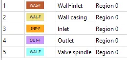
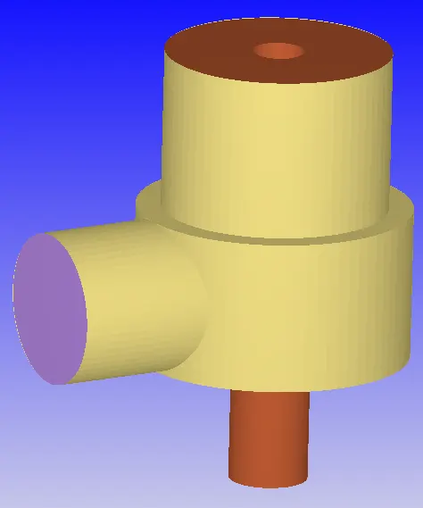
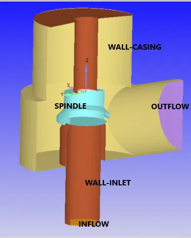
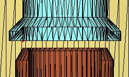
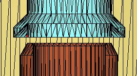
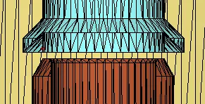
The CAD model of the valve is given as a .stl file; Geometry clean-up and flagging is done and the required fluid volume is extracted. The bounding box of the geometry is of dimensions: 0.1818 X 0.2574 X 0.2905 m. The cut section of the geometry is shown below. The geometry is modified to accommodate three different spindle lifts - 5mm, 4mm, 3mm respectively, measured from the inlet surface (brown boundary) which is also shown below.

2) Material:

Gas==> Air (compressible)

3) Mesh:

The base mesh used is 4e-3 m in all three directions. In addition, AMR is set up for the steady-state simulation. AMR is applied on the pressure with a default SGS value of 2.5 Pa and an embed level of 3. AMR is not applied to the transient simulation keeping in mind the computational resources and time required.

4) Boundary Conditions:

Inlet: 'Air' is the incoming fluid at a pressure of 30 bar and a temperature of 300K.

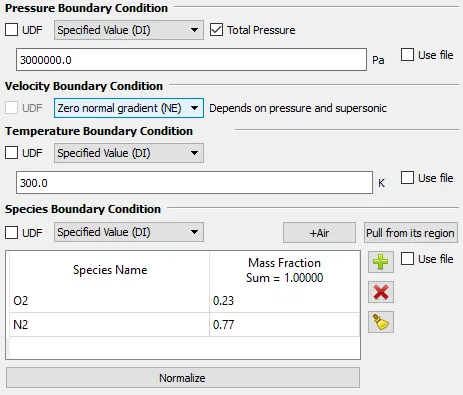
Outlet: The pressure at the outlet is fixed at a value of 1 atm (101325 Pa). In the case of backflow, the backflow species is 'air' at 300K.

Wall-inlet, Wall-casing, and Spindle: These are set as 'wall' boundary with the Law of the wall BC at 300K.

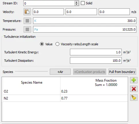
5) Initial Conditions:

The region consists of air at a temperature of 300K at 1 atm initially.

6) Simulation and Time parameters:

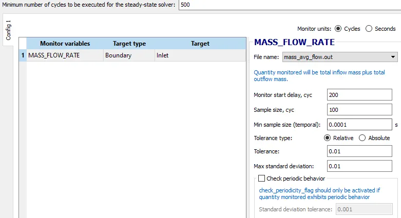
A full hydrodynamic simulation is performed with a steady-state solver. The N-S solver is set to PISO (Pressure Implicit with Splitting of Operators) which is predominantly used to handle unsteady simulations. It uses the concept of pressure correction; The algorithm uses 1 predictor step and 2 corrector steps to arrive at an accurate value for the pressure correction term. A density-based solver is chosen to deal with high-speed flows.

The end time of the simulation is considered as 15000 cycles. The CFL numbers are at their default values. A steady-state monitor is applied to the inflow mass flow rate. Hence, at convergence, the value of the steady-state pressure can be obtained at a particular value of lift.

7) Turbulence properties:

RNG `k-epsilon` turbulence model is set for the case. Generally, the standard `k-omega` SST model is suitable for capturing pressure drop. If details such as drag on impeller blades are to be captured, the `k-omega` SST turbulence model would be more suitable.

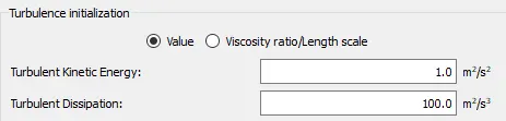
The (Initial Conditions) initial value of Turbulent Kinetic energy 'a' is assigned to the default value of 1 `m^2s^-2` and Turbulence Dissipation rate '`epsilon`' is assigned to the default value of 100 `m^2s^-3`.

8) Output/ Post processing variables reqd:

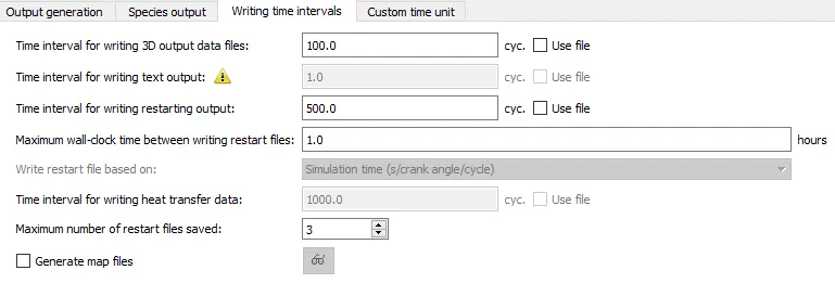
CHANGES REQUIRED IN CASE OF TRANSIENT SIMULATION:

• Firstly the geometry is modified to a spindle lift of 1mm. Next, the solver is changed to a transient mode.
• Body forces are enabled under 'simulation parameters' and gravitational acceleration of 9.81 m/s^2 is applied in the '-Z' direction.

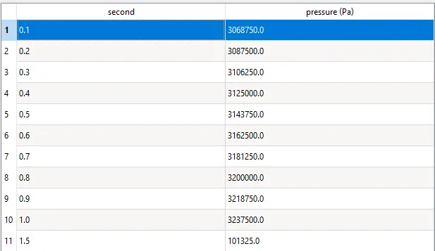
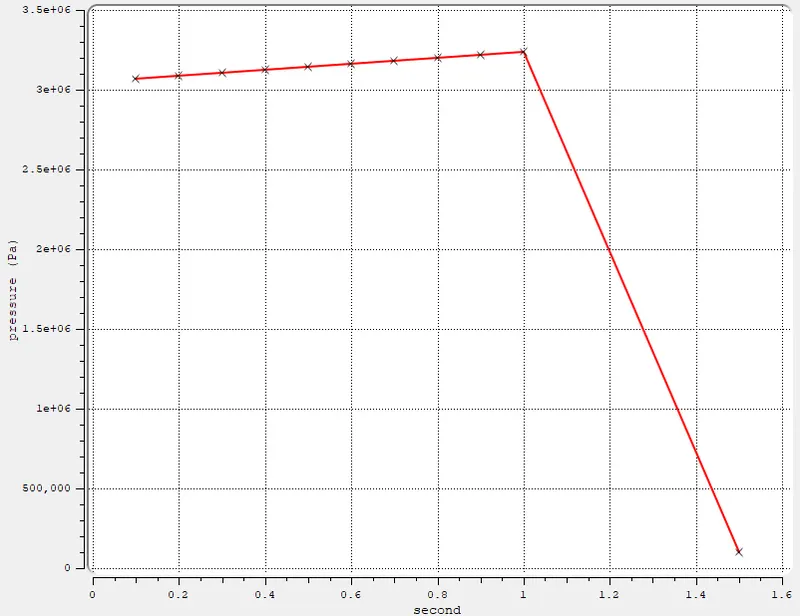
• In the transient case, pressure at inflow varies as a function of time according to the empirical function `P = (30.5 + 1.875*t)*10^5` Pa from [1]. This is provided as the inflow boundary condition as a data file: inlet_pressure.in. The plot of the varying pressure is shown below.

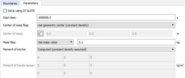
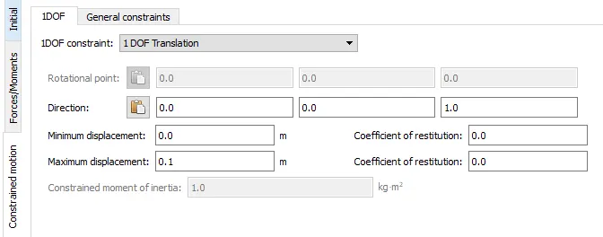
• Now, under physical models, the Fluid-Structure Interaction (FSI) is enabled. With FSI, the interaction of the spindle (structure) and the incoming air (fluid) is captured. A 'rigid FSI' is applied to the spindle boundary. Rigid FSI objects can be translated and rotated by pressure and viscous forces, but they do not change shape. The mass of the spindle is considered 3.1 kg as per [1] and is assumed of constant density. The initial tension of the spring is considered as 7126 N, as per [1]. 1 DOF motion is enabled to restrict the motion of the spindle to one direction translation. The minimum displacement is set to 0 meters and the max displacement is set to 0.1 meters which is the max distance that the spindle can travel across the sleeve. After setting up FSI, under the boundaries conditions tab in the case setup tree, the spindle wall motion is changed to type 'FSI'.

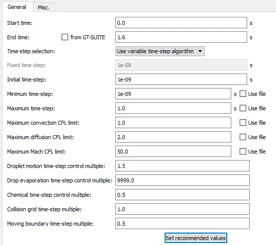
• Next, the simulation end time is to be set. The given variable pressure array is up to a time of 1.5 seconds. Hence, the simulation end time can be considered as 1.6 seconds. All other parameters and CFL numbers are kept at the default values.
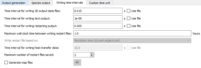
• Finally, the time at which the output files are to be captured is set. This concludes the case set up for the transient case. The simulations are run after file export.

EXPORT OF INPUT FILES:

In Converge Studio, the case set-up of the problem is done. This essentially creates all the necessary input files for the Converge solver. Once the case setup is done, the input files are exported to a new folder. Shown below is the list of input files that have been generated by Converge Studio.

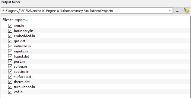
RUNNING THE SIMULATION:

A Command-line editor tool like Windows CMD or CYGWIN is used to set up the run. Here Windows CMD is used. Firstly, the location of the input files is navigated to and the Converge solver is called using the Command Line tool. For faster computational speed, parallel processing is set up on multiple cores using INTEL MPI software.

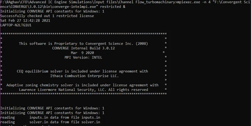
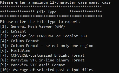
At the end of the run, the solver generates "post.h5" files (3D Output files) and ".OUT files" (Data files). The ".OUT" files contain data at mesh points. The 3D Output files are further post-processed using Converge post-processing tool into "Paraview VTK-Inline Binary format" to further analyze the case in Paraview.

RESULTS:

1) Mesh:

With AMR (left) and without AMR (right):

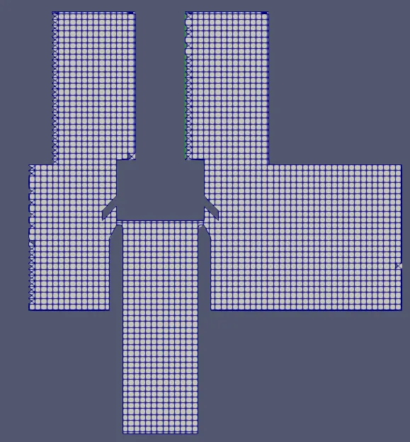
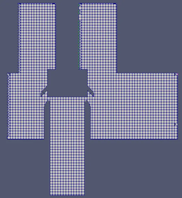
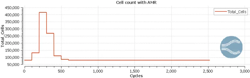
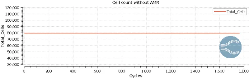
• Not many differences exist in the meshes generated with/without AMR as the meshes look similar. The number of cells at steady-state in both the cases: with and w/o AMR is ~80,000. Hence, slight variations in the captured data can be expected.
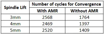
• The number of cycles in the case of 'with AMR' is 2520 at convergence and in that case of 'without AMR', is 1764 at convergence.

2) Check for convergence:

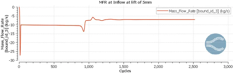
• In the steady-state simulation, the steady-state monitor was set on the mass flow rate at the inlet boundary. The plot of mass flow rate at the inlet is checked for convergence.
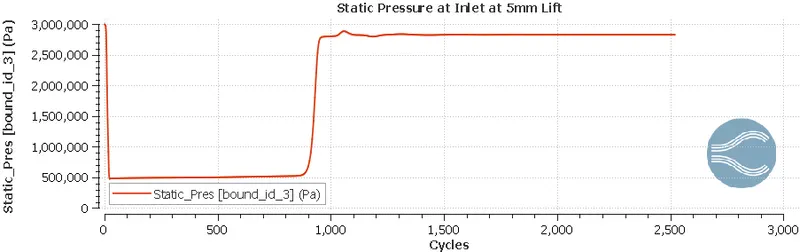
• In addition to MFR, the static pressure at the inlet is also checked for convergence.
• From the plots shown below, it is observed that the MFR and the static pressure and hence the simulation have attained convergence.
• Similar plots are obtained for lifts of 3mm and 4mm.

3) Contours and plots of Velocity and Pressure for spindle lift of 5mm:

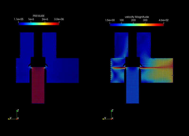
With AMR:

Without AMR:

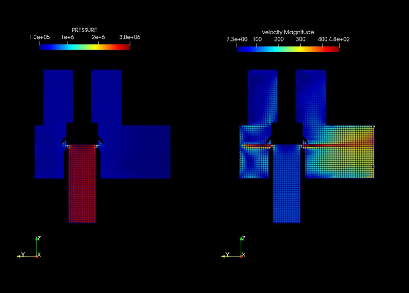
• The velocity and pressure contour are very similar for both mesh cases.
• High pressure is built along the inlet channel and at a particular lift, the flow jets itself out with massive kinetic energy normal to the inlet direction. This is shown by the velocity contour.
• The 'contour with AMR' shows lesser kinetic energy diffusion in the casing of the relief valve.
• Similar trends are observed at other lifts.

4) Plot of Pressure Force on Spindle VS Lift:

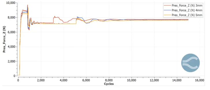
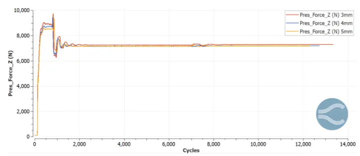
The plot of pressure force on the spindle at various lifts for the two mesh cases (with and without AMR) are shown:

A) With AMR

B) Without AMR

Inferences from the above Plots:

• From the pressure force (Z) vs Lift plot, for both mesh cases, it is observed that, as the lift increases, the pressure force acting on the spindle surface decreases. This is because more flow gets diffused into the relief valve chamber with increasing lift and the remaining liquid exert pressure force on the spindle.
• The results capture the pressure gradient more accurately when AMR is enabled and give more realistic results for pressure force.

5) Results from the Transient FSI Simulation:

a) Animation of Pressure and Velocity Contour:

• The transient behavior of the relief valve is clear from the above animation.
• With increasing pressure force, the downward spring force and the weight of the spindle are overcome and the excess pressure is relieved. Once the excess pressure is relieved, the spring force pushes back the spindle downwards and these events repeat according to the supplied pressure profile. This is how a pressure relief valve works!
• It can be noticed that even after the pressure of flow is brought to baseline pressure, the flow still exists at the relief valve casing. This is because there exists a gap in the geometry between the spindle and the inlet channel which cannot be closed without geometry intersection. Also, the entire volumetric domain is modeled as one region. No separate regions and events are specified. Hence, even after the valve lift becomes minimum, some flow keeps leaking into the relief valve casing. This can be rectified by using the regions and events concept or by using a UDF.

b) Position, Velocity, and Force Plot:

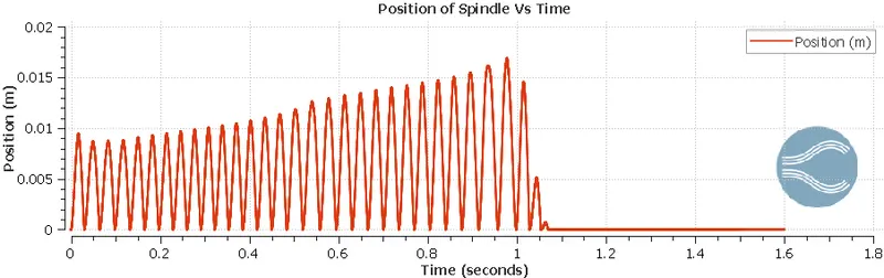
• According to the pressure profile acting on the spindle and the opposing spring force, the spindle shows oscillatory behavior. The magnitude of the position increases with increasing pressure.
• The spindle returns back to its original position after the applied pressure is back to the baseline pressure.

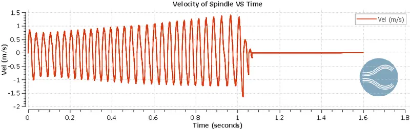
• From the velocity profile, the frequency of oscillation can be obtained to calculate the cyclic load on the valve which in turn, can be used to run a fatigue analysis using an FEA solver and hence predicting the life of the valve.
• The frequency is calculated by `f = 1/T`. It is calculated as 1/0.0167 = ~60 Hz

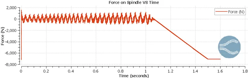
• The spring force specified on the valve is -7126 N. It can be inferred from the plot that, the hydraulic force acting on the spindle overcomes the spring force (rises over the negative regime). Beyond this, the oscillatory nature of the forces is observed.
• After 1 second, as the pressure falls, the spring force overcomes the hydraulic force and drops back to the initial tension of -7126 N on the spindle.

CONCLUSION:

The Steady-state simulation of the Safety relief valve at various lifts is conducted and a comparison plot of the pressure force acting on the spindle on various lifts is generated for both the mesh cases. It is observed that as the lift increases, the pressure force acting on the spindle decreases on the account of flow diffusion.

In the second part of the challenge, the transient FSI simulation of the Safety relief valve is performed to decipher the behavior of the valve spindle under transient inlet pressure conditions. It is found that the valve exhibits an oscillating nature on the account of upward pressure forces and the downward spring forces. With the increase in the pressure force, the amplitude of oscillation increases. Other FSI based plots such as velocity and force on the spindle are plotted wrt time.