Simulating the Prandtl Meyer Shock problem using CONVERGE

OBJECTIVE:

In this challenge, the Prandtl Meyer Expansion Waves are investigated and simulated on Converge. An investigation on the fundamentals of shockwaves is also touched upon.

AN INVESTIGATION ON FUNDAMENTALS OF SHOCKWAVES AND ITS TYPES:

Reference: Fluid Mechanics Fundamentals and Applications by Yunus Cengel, John M. Cimbala

1) Shockwave and its boundary conditions:

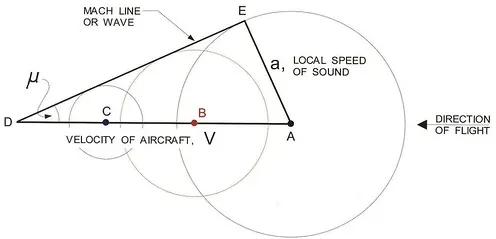
When there is a disturbance in a compressible medium due to an infinitesimal pressure difference, the disturbance travels through the medium with the speed of sound. These are pressure waves. The information/disturbance traverses through the media differently depending on the Mach number. In the case of supersonic flow, the information cannot be observed upstream but can only be perceived by the observer when he enters the region of the Mach cone.

In the case of supersonic flow, when the back pressure of the flow keeps is sufficiently decreased, a thin section of a standing wave is formed across which the properties of flow change abruptly. This thin section is called a Shockwave (Normal Shock). Post the shockwave, the flow is subsonic in nature to conserve the mass flow rate.

Across a shockwave, the entropy remains constant, but there is a spike in temperature, velocity, and Internal energy. Shockwaves are usually very thin in order of micro/millimeters. Shocks usually exist as sharp discontinuities but they can be smoothened out using lower order numerical methods. In higher-order schemes, the shocks present themselves with oscillations due to Gibbs Phenomena.

a. In Supersonic compressible flows where shockwaves exist, at the inlet usually, a Dirichlet velocity condition must be specified to make the flow supersonic. Supersonic flow PDEs are generally hyperbolic in nature.

b. Next, a 'continuative' boundary condition, zero Normal Derivative (Neumann Boundary condition) is generally preferred at the outlet. This boundary condition is intended to make a smooth continuation of flow through the boundary. The value of the parameters at the boundary is extrapolated with space and time marching.

2) Types of Shockwaves:

1. Normal Shock
2. Oblique Shock
3. Bow Shock
4. Prandtl Meyer Expansion Wave

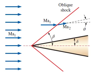
Shown above is a representation of an oblique shockwave. Here `delta` is the wedge angle (Angle made by a 2D Object). `theta` is the deflection angle i.e. the angle by which the flow turns across the shock to ensure the conservation of mass. `beta` is the shock angle. The red line is the oblique shock.

Normal shock can be visualized as an Oblique shock with `beta` = 90 deg

3) Prandtl Meyer Expansion Waves:

Expansion Waves: Expansion waves appear when the turn angle does is not against the flow. This may result in the formation of Mach Waves.

Compression Waves: Compression waves appear when the turn angle is against the flow and it results in oblique shock.

Mach Waves: The weakest possible oblique shock (`beta = betaunderset(min)()` ) at a particular Mach number is called Mach Wave.

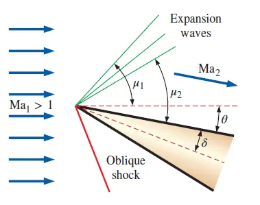
In the Prandtl Meyer Expansion Fan, as it is called, there exists a continuously expanding region, an expansion fan which is a cluster of an infinite number of Mach waves, each one turning the direction of flow by an infinitesimal amount. This means flow does not abruptly change its direction like a shockwave but it happens gradually. If the angle of turn of the flow is known, the Mach number can be calculated using the relation:

where `mu` is called Mach Angle obtained by applying `theta = 0` and `beta = mu`; Across the Prandtl Meyer Expansion fan, the Mach Number increases, and other properties such as Pressure, Temperature, and Density decrease.

CASE SET-UP IN CONVERGE STUDIO:

In this project, a Prandtl-Meyer expansion fan is simulated using Converge. The given geometry in form of .stl file is imported into Converge. The geometry consists of a sharp convex turn required for the generation of the expansion fan.

1) Geometry:

The geometry bounding box is of dimensions 65m X 45m X 8m.

2) Mesh:

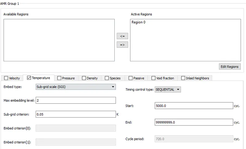
The mesh sizes used are 0.8m in all three directions. The Adaptive Mesh Refinement (AMR) option has been enabled. AMR takes in the type of embed which is selected as 'Semi Grid Scale (SGS)'. SGS refines the mesh size when the curvature (2nd order derivative) of the parameter on which it is applied goes beyond the sub-grid criterion. AMR can be applied to any of the flow parameters such as velocity, pressure, or temperature.

Here, AMR is applied to temperature and it is enabled in region0. The max embedding level is set to 2. The sub-grid criterion is set to 0.05. This means whenever the SGS temperature difference goes beyond 0.05K, mesh refinement takes place. The maximum refinement of SGS is `0.8/2^2 = 0.2` [`Grid size = (base grid)/(2^(embed)`]

3) Material:

Gas ==> Air

4) Boundary Conditions:

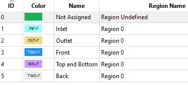
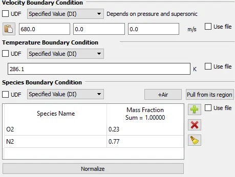
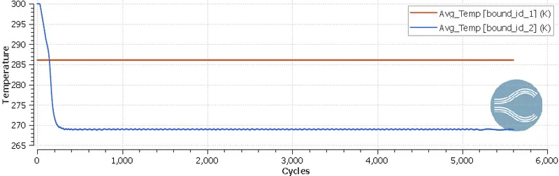
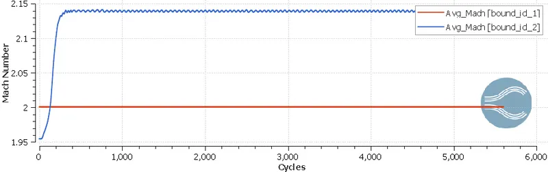
Inflow Boundary Condition: A Dirichlet BC is applied at Inflow. The Velocity of air is set to 680m/s in x-direction at a temperature of 286.1K. At this temperature, the velocity of sound is ~340m/s. This means the inlet Mach number is 2.

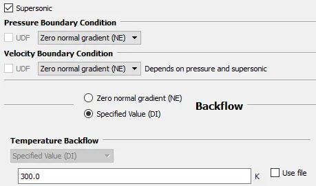
Outflow Boundary Condition: Pressure and Velocity set to Neumann BC.

Top & Bottom: Wall Boundary Condition: Wall with slip boundary condition

TWO_D Boundary Condition: Two_D BC is applied to the Front and Back of geometry to ensure a 2D simulation.

5) Initial Conditions:

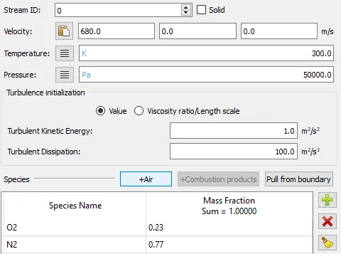
Species of Air at 680m/s, temperature of 300K and Pressure of 50000 Pa.

6) Simulation and Time parameters

A full hydrodynamic simulation is performed with a steady-state solver. Steady-state solver implies that irrespective of the path of the process and the initial conditions, the simulation will reach steady-state and give tangible results as long as the geometry and boundary conditions are given right.

The N-S solver is set to PISO (Pressure Implicit with Splitting of Operators) which is predominantly used to handle unsteady simulations. It uses the concept of pressure correction; The algorithm uses 1 predictor step and 2 corrector steps to arrive at an accurate value for the pressure correction term. The solver type is set to Density-based as the problem deals with high-speed compressible flows.

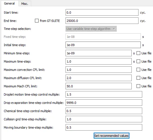
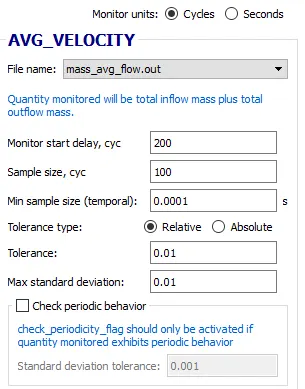
Simulation start time is 0 cycles and end time is 25000 cycles. It is controlled by a steady-state solver monitoring velocity at exit. The steady-state monitoring starts functioning after 500 cycles and once the average parameter (avg. velocity in this case) attains steady-state, the simulation is shut off. The average is calculated by taking sample data of a specified size (100 in this case). The relative tolerance limit set for a sample size of 100 cycles is 0.01.

7) Turbulence properties:

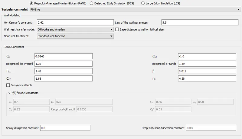
RNG `k-epsilon` turbulence model is set for the case. Generally, the standard `k-omega` SST model is used at the industrial level. Not many differences exist between RNG `k-epsilon` and the `k-omega` SST model.

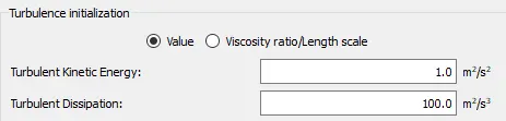
The (Initial Conditions) initial value of Turbulent Kinetic energy 'k' is assigned to the default value of 1 `m^2s^-2` and Turbulence Dissipation rate '`epsilon`' is assigned to the default value of 100 `m^2s^-3`.

The basic idea of the RNG `k-epsilon` model is to solve the transport equations involving Turbulent Kinetic energy 'k' and Turbulence Dissipation Rate '`epsilon`' to arrive at the values of k and `epsilon`. With the values of k and `epsilon`, the Eddy viscosity can be calculated. With the value of Eddy viscosity, the Reynolds stresses, and further, the RANS equation can be solved for average velocity. Shown below are the default RANS constants which are to be used in the k-`epsilon` transport equation.

8) Output/ Post processsing:

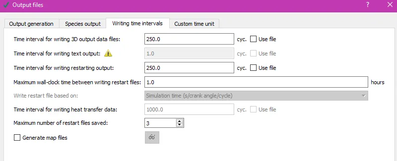
The post-run data variables selected are Pressure, Temperature, Velocity, and Density, Dissipation Rate (`epsilon`), Turbulent KE (k), Turbulent viscosity. The time interval of writing 3D Output files and text files are set such that 100 data files of each are generated. The time interval for restart files is the same as that of 3D output.

EXPORT OF INPUT FILES:

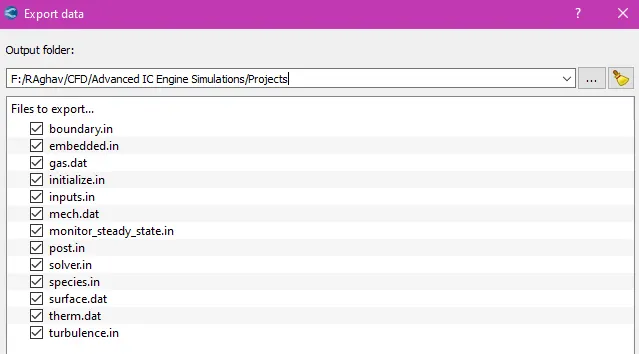
In Converge Studio, the case set-up of the problem is done. This essentially creates all the necessary input files for the Converge solver. Once the case setup is done, the input files are exported to a new folder. Shown below are the input files that have been generated by Converge Studio.

RUNNING THE SIMULATION:

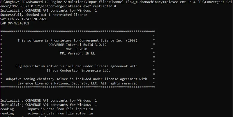
A Command-line editor tool like Windows CMD or CYGWIN is used to set up the run. Here Windows CMD is used. Firstly, the location of the input files is navigated to and the Converge solver is called using the Command Line tool. For faster computational speed, parallel processing is set up on 4 cores using INTEL MPI software.

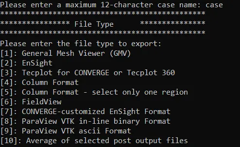
At the end of the run, the solver generates "post.h5" files (3D Output files) and ".OUT files" (Data files). The ".OUT" files contain data at mesh points. The 3D Output files are further post-processed using Converge post-processing tool into "Paraview VTK-Inline Binary format" to further analyze the case in Paraview.

RESULTS:

Mesh:

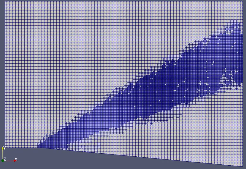
It can be observed that initially the mesh whose size is 0.8m in all directions, has been refined near the shock location. Near the expansion fan, refinement has occured. The minimum cell size after refinement is `0.8/2^2 = 0.2 m`

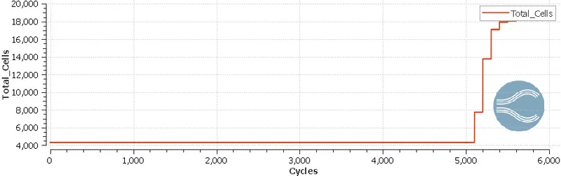
Avg Number of Cells Plot:

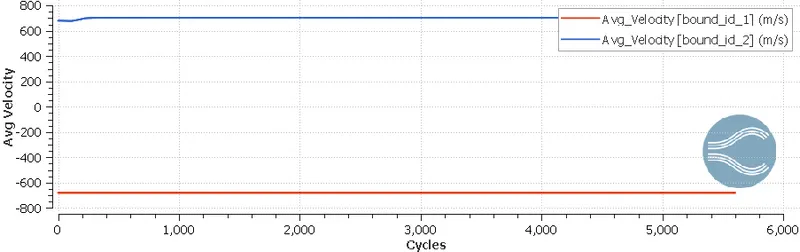
Velocity Plot at 0.01 SGS:

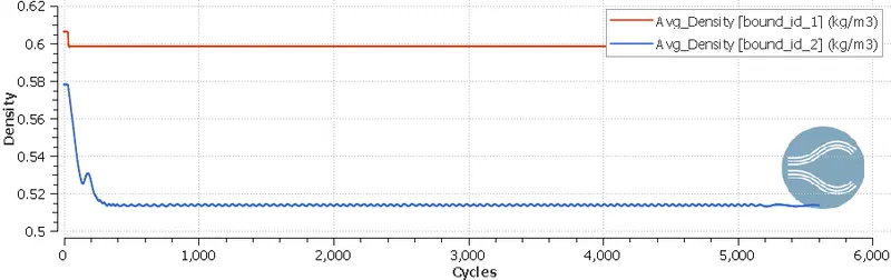
Density Plot at 0.01 SGS:

Temperature Plot at 0.01 SGS:

Avg Mach Number Plot at 0.01 SGS:

Animation of Temperature Contour of Prandtl Meyer Expansion Fan:

INFERENCE and CONCLUSION:

1. The simulation runs ~5600 cycles after which it reaches a steady state.
2. The initial cell count is ~4000. The max cell count at the end of the simulation is ~18000. This is attributed to Adaptive Mesh Refinement (AMR).
3. The Mach Number at the Inlet is 2. The Mach number post the expansion fan is ~2.14. This is a valid result as it is known that the Mach number increases across the expansion fan.
4. The velocity at the inlet is 680 m/s and at the outlet, it is extrapolated to ~700 m/s. This result is in accordance with the increase in Mach Number.
5. From the density plot, it can be observed that density decreases from ~0.59 to ~0.51. Post the expansion fan, the flow behaves just like the diverging part of the Convergent Divergent Nozzle. With acceleration in velocity, pressure decreases and this decreases the density at the outflow.
6. The temperature decreases across the expansion fan from 286K to 269K.
7. The pressure decreases from 386649 Pa at the inflow to 386057 Pa at the outflow.

Effect of SGS parameter on Cell count:

It can be seen that for SGS of 0.01 the total no of cells generated is ~18000. For SGS of 0.05, the total number of cells is ~7000 and the cell count is ~5000 for SGS of 0.1. It is clear from these results that, as the SGS parameter decreases, the more is the refinement and more will be the number of cells. This increases the accuracy of the solution but would result in an increase in resources consumed. If SGS is not high enough, AMR will not make any difference as grid independence will be reached. If SGS takes a very high value, it would be as good as no AMR applied as the tolerance limit set is very high.

Effect of SGS parameter on Location of shock:

A) Shock Location @ 0.01 SGS captured at Steady State

B) Shock Location @ 0.05 SGS captured at Steady State

C) Shock Location @ 0.1 SGS captured at Steady State

It is observed that as the SGS factor increases, the expansion fan increases in bandwidth. At an SGS of 0.01, the shock is captured accurately. At an SGS of 0.05, we can see that the bandwidth of the Mach waves has increased. And further, at 0.1 SGS, it can be observed that the light blue region and the red region have expanded more.

It is better to keep SGS at a lower value as a more accurate solution can be obtained in terms of shock bandwidth and characteristic parameters. If the SGS is set to a high value, it is as good as 'AMR not making a difference' since all the curvature values would not fall within the set limit.