Centrifugal pump simulation using Converge

OBJECTIVE:

In this challenge, a transient simulation of flow through a centrifugal pump is carried out using Converge. The performance curve of the pump is plotted and the efficiency of the pump is calculated at various mass flow rates.

It is to be noted that the effects of cavitation are not considered in this challenge as the simulation with 2 phase flow and a moving mesh would demand huge computational resources.

SOFTWARES USED:

1. Converge Studio v3.0
2. Windows CMD and CYGWIN
3. Paraview

BRIEF WORKING OF A CENTRIFUGAL PUMP:

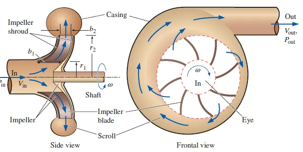
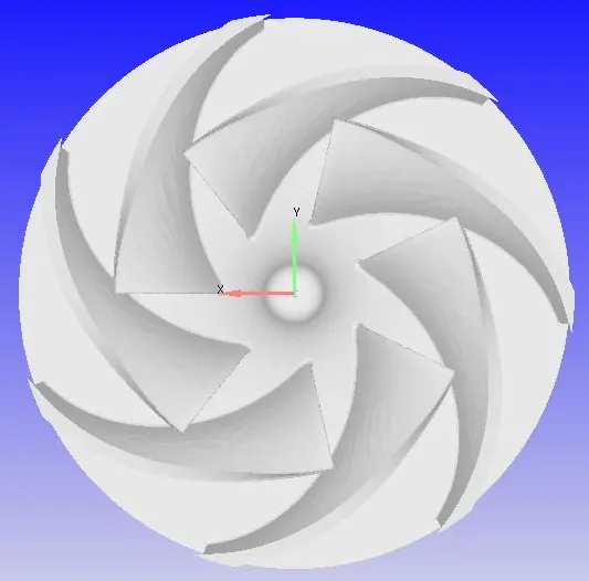
A centrifugal pump is a type of dynamic pump that constitutes of rotating blades that imparts momentum change to the flow. Centrifugal pumps have a snail-like casing called the volute or scroll. The rotating components (impeller blades, impeller shroud, and impeller sweep) as a whole are termed the Impeller. The fluid enters through the eye (axially) to the rotating blades and exits radially through the casing.

The work done on the pump under ideal conditions is equal to the momentum change imparted by the rotating blades on the fluid. The momentum transfer brings a change in the radial and tangential components of velocity of flow. In addition, the centrifugal force causes an increase in the radial velocity of flow.

Usually, there exists an increasing cross-section between the blades of the impeller which causes a pressure rise in the flow. As the fluid flows through the volute, the fluid leaving the blade is decelerated and channeled to a common exit. In this process, the fluid becomes further pressurized. The resulting flow at the outlet is highly pressurized and there may or may not be a velocity rise depending on the diameter of the inlet and outlet.

CASE SETUP IN CONVERGE STUDIO:

1) Geometry and flagging:

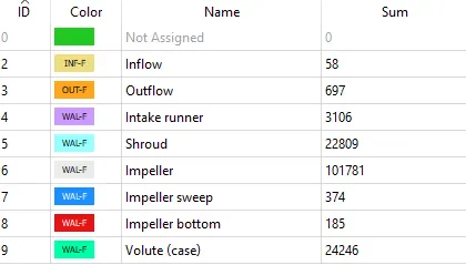
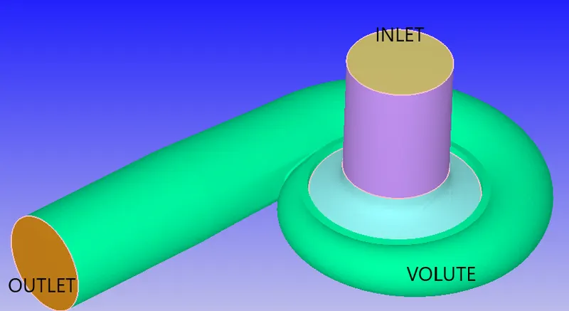
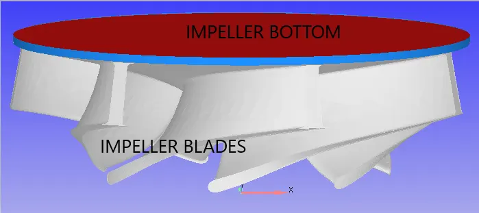
The given Geometry is a .stl file. It is imported into Converge. Geometry clean-UP and boundary flagging are carried out initially. The bounding box of the geometry is of dimensions 0.8917m X 0.5959m X 0.3960m

2) Mesh:

The base mesh sizes used are 0.012m or 12 mm in all three directions.

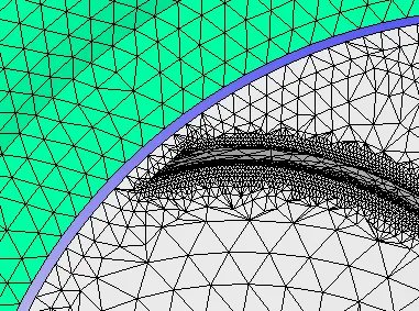
To come up with the right mesh embedding at the impeller, the location of the least fluid volume is to be determined. It is found that this minimum distance (shown below) is ~0.002m or 2mm. It is of prime importance to have at least one cell in this small gap to capture the velocity and pressure gradients accurately. A mesh scale factor of 12/2 = 6 is the ideal choice. But with this choice of mesh size, considering the moving nature of the mesh, the computational time is found to extend for ~6 days on a 16-core CPU. Also, in another test case, with an embed mesh scale of 2 i.e. with the smallest cell size of 3mm, the results obtained were almost similar to the case with finer mesh at steady-state. Hence, a base grid of 12mm with an embed scale of 2 is selected and applied to Impeller, Impeller bottom, and Impeller sweep.

3) Material:

Liquid ==> Water

4) Boundary Conditions:

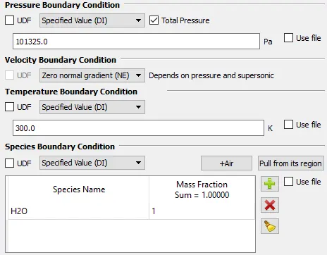
Inlet: Water at a total pressure of 101325 Pa and a temperature of 300K. NPSH is not considered as the effects of cavitation are neglected.

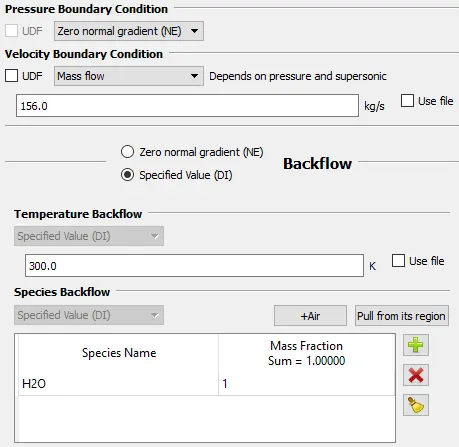
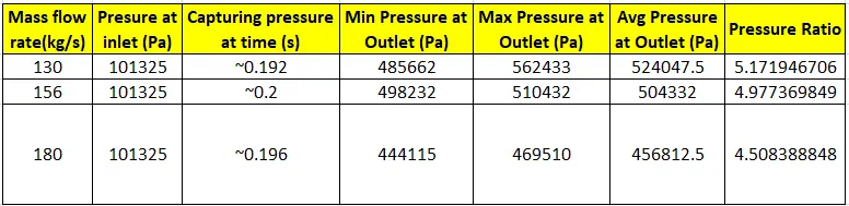
Outlet: The mass flow rate is specified at the outlet. For a 20mm diameter of the impeller, the tangible mass flow rates range from 120 to 200 kg/sec. Three mass flow rates are selected and the simulation is carried out for the 3 cases in order to plot a performance curve. The various mass flow rates are 130 kg/sec, 156 kg/sec and 180 kg/sec.

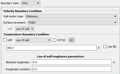
Intake runner, shroud, and volute: The intake runner and shroud are specified as a wall with the Law of Wall boundary condition.

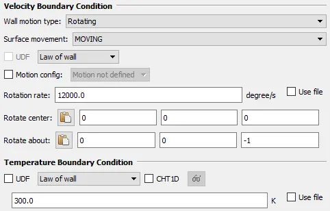
Impeller, Impeller sweep, and Impeller bottom: The impeller and its components are specified as a Rotating wall at a rate of 12000 deg/sec with the Law of the wall boundary condition.

5) Initial Conditions:

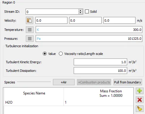
Water present at 300K and 101325 Pa.

6) Simulation and Time parameters:

The simulation to be carried out is a pure liquid simulation. The pump only deals with subsonic flow speeds and hence the liquid flow solver is set to incompressible. A full hydrodynamic simulation is performed with a transient solver. The N-S solver is set to PISO (Pressure Implicit with Splitting of Operators) which is predominantly used to handle unsteady simulations. It uses the concept of pressure correction; The algorithm uses 1 predictor step and 2 corrector steps to arrive at an accurate value for the pressure correction term. Pressure based solver is chosen to deal with low-speed flows.

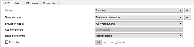
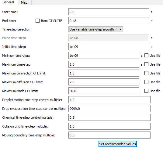
The time parameters are shown below: Simulation start time is 0 sec and end time is 0.18 sec. The impeller must rotate 2-6 times to reach a steady or pseudo steady state.

End Time Calculation:

360 degrees per sec ==> 1 rps

`implies` 12000 degrees per sec = 33.33 rps

i.e. 33 rotations ==> 1 sec

`implies` 6 rotations = 0.18 sec

7) Turbulence properties:

RNG `k-epsilon` turbulence model is set for the case. Generally, the standard `k-omega` SST model is suitable for capturing pressure drop. If details such as drag on impeller blades are to be captured, the `k-omega` SST turbulence model would be more suitable.

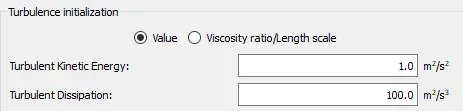
The (Initial Conditions) initial value of Turbulent Kinetic energy 'a' is assigned to the default value of 1 `m^2s^-2` and Turbulence Dissipation rate '`epsilon`' is assigned to the default value of 100 `m^2s^-3`.

8) Output/ Post processsing:

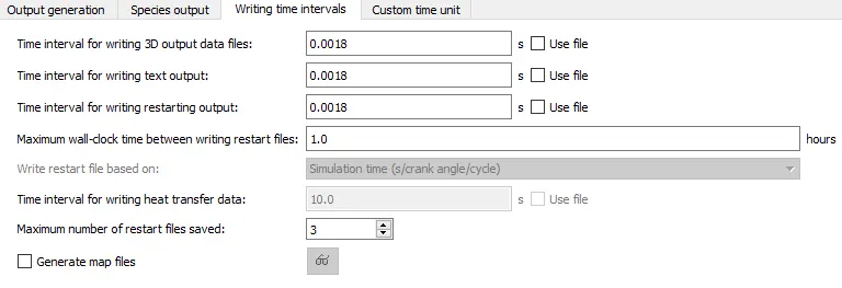
The post-run data variables selected are Pressure, Temperature, Velocity, and Density, Dissipation Rate (`epsilon`), Turbulent KE (k), Turbulent viscosity. The time interval of writing 3D Output files and text files are set such that 100 data files of each are generated. The time interval for restart files is the same as that of 3D output.

EXPORT OF INPUT FILES:

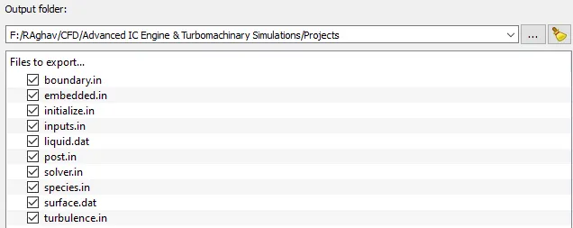
In Converge Studio, the case set-up of the problem is done. This essentially creates all the necessary input files for the Converge solver. Once the case setup is done, the input files are exported to a new folder. Shown below is the list of input files that have been generated by Converge Studio.

RUNNING THE SIMULATION:

A Command-line editor tool like Windows CMD or CYGWIN is used to set up the run. Here Windows CMD is used. Firstly, the location of the input files is navigated to and the Converge solver is called using the Command Line tool. For faster computational speed, parallel processing is set up on multiple cores using INTEL MPI software.

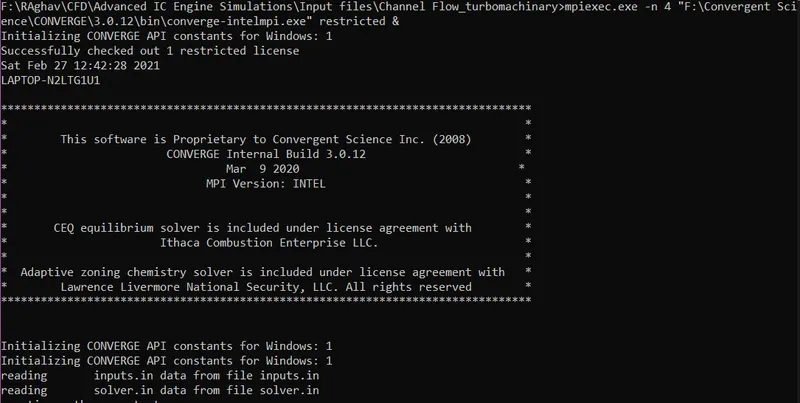
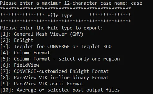
At the end of the run, the solver generates "post.h5" files (3D Output files) and ".OUT files" (Data files). The ".OUT" files contain data at mesh points. The 3D Output files are further post-processed using Converge post-processing tool into "Paraview VTK-Inline Binary format" to further analyze the case in Paraview.

RESULTS:

Mesh:

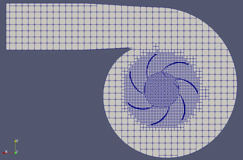
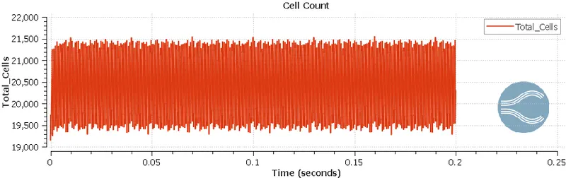
A no-hydro simulation is performed with a coarse mesh and mesh embedding. This mode of simulation ignores the transport equations to greatly reduce the computational time and is an efficient way to check for errors in the surface motion and mesh creation. The max cell count is ~21500.

Plotting the Performance Curve:

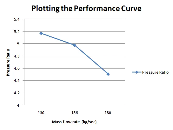
The performance plot is obtained by plotting the Net Head across pump VS Mass Flow Rate of the pump. Since this challenge works on low velocities of flow and a small height difference, these values can be neglected. The Net Head gain across the pump is directly dependant on the Pressure ratio obtained. Hence, the performance plot is essentially a Pressure Ratio VS Mass Flow Rate curve.

*It is necessary to note that this challenge only focuses on capturing the trend of the performance chart and the result obtained cannot be validated as neither the real-time data from a pump manufacturer nor a real-time 3D CAD model of a pump is available.

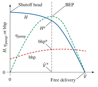
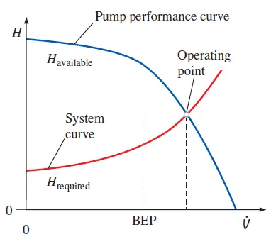
Shown below is a reference plot of a centrifugal pump performance curve obtained from Cengel. The volume flow rate or mass flow rate (X-axis) is maximum at 0 Head (Free delivery) condition where there is no resistance to flow. The max head is obtained when the flow from the pump is blocked. The best efficiency point (BEP) is the max efficiency of the pump and is obtained somewhere between zero volume flow rate and free delivery. The steady-state working of the pump is obtained when the head required by the system is matched with the head available. This point is known as Operating Point and must be as close to BEP as possible.

The pressure at the inlet is known: 101325 Pa. The total pressure at the outlet can be obtained from the mass_avg_flow.out file. Shown below is the pressure plot for a mass flow rate of 156 kg/sec.

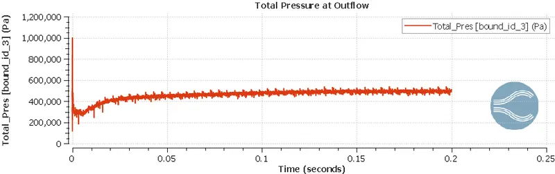
At the mentioned timestep, the average pressure at Outlet is calculated by averaging the peak and crest of pressure values. The pressure ratio is then calculated corresponding to each mass flow rate as shown below. Now the performance curve can be plotted (shown below). A similar trend as that of the reference curve is being observed.

Calculation of Pump Efficiency:

The efficiency of a pump is given by:

-------------------------------------(A)

where the symbols represent the standard terms. `omega` represents the rotational speed of shaft in radian/sec and `Tunderset(shaft)()` represents the torque supplied to the shaft. The Net Head Gain (H) is calculated using the Bernoulli equation. Losses are neglected.

-------------------------------------(B)

From the plots, the required values of pressure (already calculated) and velocity at the Inflow and Outflow can be estimated. The height difference between the center of the Inflow boundary and Outflow boundary is measured in Converge studio and is found to be 0.30856 m. Hence all terms of the Bernoulli equation are known.

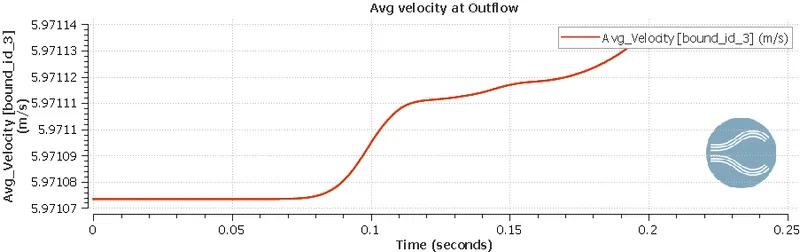
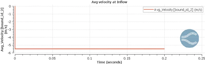
The net head gain is now calculated corresponding to each value of mass flow rate using equation (B):

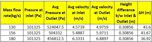
The numerator of the pump efficiency can now be calculated. Now the task is to calculate the denominator. `omega` is calculated by multiplying 12000 deg/sec with `pi/180`. The torque acting on the shaft is obtained from the 'Pressure Torque' plot on Impeller flagged boundary file. It is to be noted that the torque on the shaft acts along the Z-axis and the file corresponding to Z-axis torque must be used. Shown below is the pressure torque plot for a mass flow rate of 156 kg/sec.

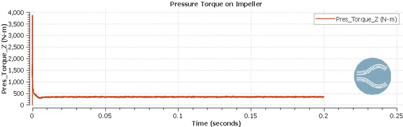
Now, the efficiency of the pump can be calculated using equation (A). An increasing trend in efficiency is observed meaning the efficiency curve is approaching the BEP point.

Animation of Velocity and Pressure contours for MFR of 156 kg/sec:

INFERENCES FROM THE CHALLENGE:

1. The max number of cells is ~21500 with a fixed mesh embedding applied to the impeller.
2. The velocity of flow at the vicinity of the blades is maximum and it decreases as it flows through the volute. The purpose of the volute is to reduce convert the high velocity to pressure and to channelize the flow to a common outlet. It is also observed that the velocity of the flow is similar at the inlet and outlet.
3. The pressure is minimum at the eye of the impeller where the flow enters the pump and gets pressurized along with the casing. The flow exits the pump at high pressure. Hence the flow gets pressurized but the velocity at inlet and exit are close and comparable.
4. The pressure ratio or the Net Head Gain decreases with an increase in the mass flow rate.
5. The increasing efficiency of the pump indicates that the BEP is not yet attained and the difference in magnitude of the efficiency indicates that the pump is close to the BEP at a mass flow rate of 180 kg/sec.
6. The overall trend of a centrifugal pump is captured in this simulation and can be visually validated up to a certain extent.

References:

Fluid Mechanics Fundamentals and Applications by Yunus Çengel, John M. Cimbala