Transient simulation of flow over a throttle body using CONVERGE

OBJECTIVE:

In this challenge, a transient simulation of flow through an elbow-shaped channel containing a throttle plate is carried out using Converge. The challenge has two parts to it - The Steady-state simulation and Transient state simulation. The steady-state deals with the case where the throttle plate is at rest and the transient state simulation deal with a predefined motion of the throttle plate.

SOFTWARES USED:

1. Converge Studio v3.0
2. Windows CMD and CYGWIN
3. Paraview

CASE SETUP IN CONVERGE STUDIO:

The Geometry is given in form of a .stl file. It is then is imported into Converge. The thickness of the elbow body is of no interest and hence the outer wall of the geometry is removed.

1) Geometry:

The bounding box of the geometry is given by 0.106m X 0.12m X 0.017m

2) Mesh:

The mesh sizes used are 0.002m in all three directions with fixed embedding near the throttle plate.

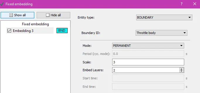
For greater accuracy, Mesh Embedding is enabled at the Inlet and Outlet boundaries. The embed mode is set to Permanent. This means the finer mesh will be present throughout the entire simulation. The Embedding scale is set to 3 and Embed layers are set to 2. The size of the cells in the embed region is given by `frac{base grid}{2^(scal e)`. Embed Layers of 2 means there would be 2 layers of such embedded mesh.

3) Material:

Gas ==> Air

4) Boundary Conditions:

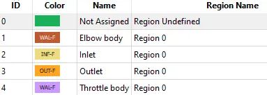
Inflow Boundary: Total pressure of 1.5 bar at a temperature of 300K and species of air entering the channel.

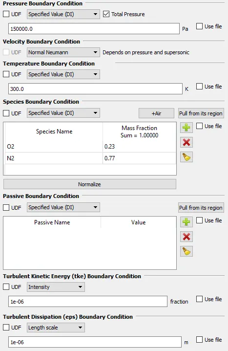
Outflow: Static pressure of 1bar with species backflow of air at backflow temperature of 300K.

Elbow Body: Wall with No-slip boundary condition

Throttle Body: Wall Boundary Condition with Rotation. The Rotation center and rotation axis are found by finding the arc center and normal of the cylinder-like projection of the throttle plate.

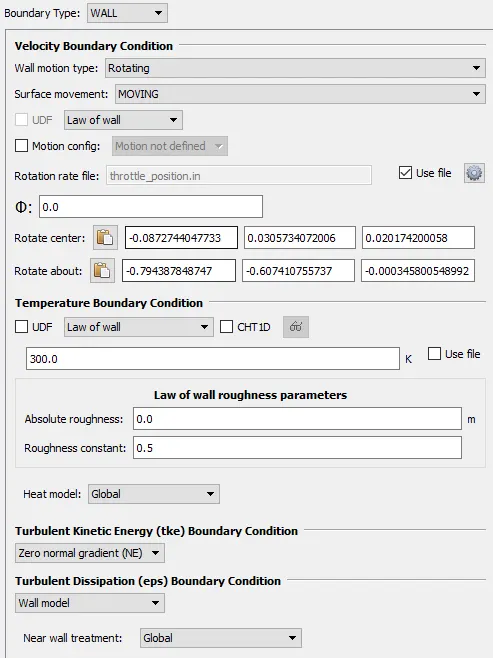
The throttle plate rotates according to the profile given below. The rotation rate file is given as input.

• 0 to 25 deg in 0.002 s
• Stay at 25 deg till 0.004 s
• Return back to 0 deg by 0.008 s
• Stay at the same position for the rest of the simulation

5) Initial Conditions:

Species of air present at 300K and 101325 Pa.

6) Simulation and Time parameters:

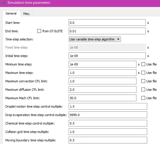
Transient simulation deals with start time and end time in seconds rather than cycles. The start time is 0 sec. The end time is calculated as the time required for the flow to pass through the entire domain 4 times.

END TIME CALCULATION:

Effective length of domain = 0.2m

Avg steady state Inlet velocity = 80 m/s

End time = Time required for flow to pass through the domain 4 times = `4*(0.2/80) = 0.01 sec`

Hence,

Start time: 0 seconds

End time: 0.01 seconds

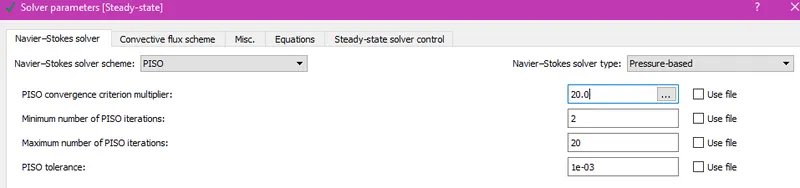
The N-S solver is set to PISO (Pressure Implicit with Splitting of Operators) which is predominantly used to handle unsteady simulations. It uses the concept of pressure correction; The algorithm uses 1 predictor step and 2 corrector steps to arrive at an accurate value for the pressure correction term.

7) Turbulence properties:

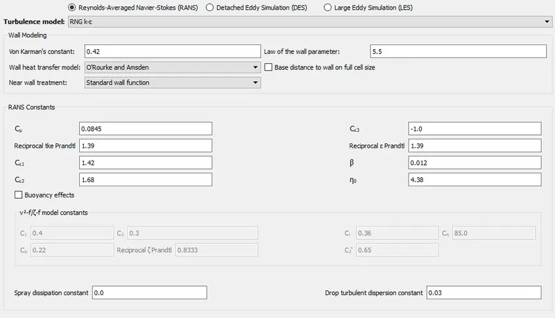
RNG `k-epsilon` turbulence model is set for the case. Generally, the standard `k-omega` SST model is used at the industrial level. Not many differences exist between RNG `k-epsilon` and the `k-omega` SST model.

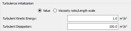
The (Initial Conditions) initial value of Turbulent Kinetic energy 'k' is assigned to the default value of 1 `m^2s^-2` and Turbulence Dissipation rate '`epsilon`' is assigned to the default value of 100 `m^2s^-3`.

The basic idea of the RNG `k-epsilon` model is to solve the transport equations involving Turbulent Kinetic energy 'k' and Turbulence Dissipation Rate '`epsilon`' to arrive at the values of k and `epsilon`. With the values of k and `epsilon`, the Eddy viscosity can be calculated. With the value of Eddy viscosity, the Reynolds stresses, and further, the RANS equation can be solved for average velocity. Shown below are the default RANS constants which are to be used in the k-`epsilon` transport equation.

8) Output/ Post processsing:

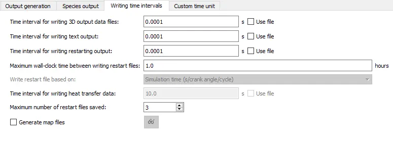
The post-run data variables selected are Pressure, Temperature, Velocity, and Density, Dissipation Rate (`epsilon`), Turbulent KE (k), Turbulent viscosity. The time interval of writing 3D Output files and text files are set such that 100 data files of each are generated. The time interval for restart files is the same as that of 3D output.

EXPORT OF INPUT FILES:

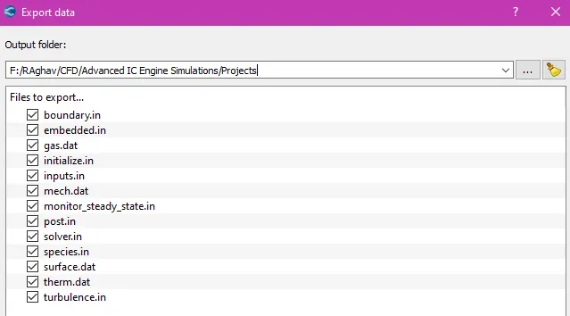
In Converge Studio, the case set-up of the problem is done. This essentially creates all the necessary input files for the Converge solver. Once the case setup is done, the input files are exported to a new folder. Shown below are the input files that have been generated by Converge Studio.

RUNNING THE SIMULATION:

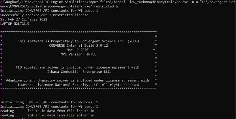
A Command-line editor tool like Windows CMD or CYGWIN is used to set up the run. Here Windows CMD is used. Firstly, the location of the input files is navigated to and the Converge solver is called using the Command Line tool. For faster computational speed, parallel processing is set up on 4 cores using INTEL MPI software.

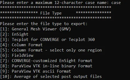
At the end of the run, the solver generates "post.h5" files (3D Output files) and ".OUT files" (Data files). The ".OUT" files contain data at mesh points. The 3D Output files are further post-processed using Converge post-processing tool into "Paraview VTK-Inline Binary format" to further analyze the case in Paraview.

RESULTS:

Mesh size: 0.002m

The mesh embed automatically comes into play according to the movement of the throttle plate. During the rotation of the throttle plate, the number of cells generated increases. During dwell time, the number of cells remains constant and decreases during returning of the throttle plate to the original position. This is shown in the video below:

Number of Cells:

Mass Flow Rate Plot:

Velocity Plot:

Pressure Plot:

Animation of Velocity and Pressure contours:

Animation of streamlines of the flow colored by the magnitude of Velocity

INFERENCE:

FROM PLOTS

1. The simulation runs for 0.01 seconds. The variation of cells is in the range of ~35000 and ~40,000. This is depicted by the total cell plot. There is an increase in the number of cells when the throttle rotates, remains constant when the throttle dwells, and decrease when the throttle comes back to its initial position
2. The velocity and the Mass flow rate plot show similar trends. There is a spike in the velocity diagram at the outlet condition because the stagnated flow now flows. There is a spike in velocity at the Inlet boundary during transience due to the effect of hammer blow due to the closure of the throttle plate.
3. The mass flow rate oscillates due to transience and converges to 0.04 kg/s at the inflow boundary increase and converges ~0.04 kg/sec
4. The static pressure shows oscillations due to the transient positions of the throttle plate. As the throttle rotates to 25-degree angle, it obstructs more fluid and this increases the stagnation pressure of the flow near the throttle. Static pressure at the outlet boundary remains unaffected.
5. The total pressure increases at the Outlet boundary when the throttle rotates to 25 deg; as the throttle rotates back to the original position, the rate of rotation is slow and does not affect the total pressure much. Total pressure remains unaffected at the inlet.

FROM CONTOURS AND STREAMLINES

1. From the velocity contour, it can be observed that velocity is initially zero. As the throttle rotates to 25deg, a max velocity of 150m/s is obtained at the outlet boundary. The case attains an intermediate steady-state during the dwell time of the throttle plate; There is a low-velocity region formed right before the throttle plate. This is called flow stagnation.
2. The same can be observed from the streamlined plot which gives a more clearer representation.
3. From the pressure contour it can be understood that as the throttle plate rotates to 25deg, the upstream gets pressurized. The region downstream to the throttle plate is a low-pressure region due to flow separation. As the throttle returns to the initial position, the pressure gets distributed along the whole pipe in a graded manner with high pressure at Inlet and low at Outlet.