Week - 2 - Explicit and Implicit Analysis
AIM:
To slove the equation F(u) = u3+9u2+4u by using both explicit and implicit methods with the tolerence of 0.001.
Explicit Analysis:
In Explicit analysis mostly dynamic analysis and nodal accelerations are solved directly (not iteratively) as the inverse of the diagonal matrix times the net nodal force vector where net nodal force includes contributions from exterior sources(body forces,applied pressure,contact etc),element stress,damping,bulk viscosity,and hour glass control.once accelerations are known at time n,velocities are calculated at time (n+1)/2,and displacements at time n+1.strain can be calculated from displacements and stress will come from strain and the cycle repeated.
Explicit analysis handles nonliniarities with relative ease as compared to implicit analysis.This would include treatment of contact and material nonlinearities.with this method is that you need many small increments for good accuracy and it is time consuming.
The nonlinear force versus displacement relationship is not known, but the stiffness is known, it is possible to construct the graph of force versus displacement numericall`
It can be done using an increment explicit load control scheme
The following equation is solved using the explicit method as follows,
`F(u)=u^3+9u^2+4u`F(u)=u3+9u2+4u"> --------(1)
Use this equation and solve using both Explicit and Implicit methods that have tolerance of 102">10^2.
Differentiating force with a request to displacement gives the stiffness (k) of the bar (since F=kx)
`k(u)=(df)/(du) = 3u^2+18u+4`---------(2)
Variables are as given below;
- U=Displacement">U=Displacement
- F = External force
- K = Stiffness
- Δu=">Δu= Incremental Displacement
- ΔF=">ΔF= Incremental externally applied force
Here, three equal load increments (or steps) of ΔF=1">ΔF=1 unit of each used to load the tension bar
STEP: 1
`u_0=0`
`k(u_0)=3(0)^3+18(0)^2+4(0) = 4`
Now,
`Deltau_1=(Deltaf)/(k(u_0)) =1/4 = 0.25`
`u_1=u_0+Deltau_1 = 0.25`
`F_(External) = DeltaF=1;`
`F_(Internal)=u_1^3+9u_1^2+4u_1=(0.25)^3+9(0.25)^2+4(0.25)=1.5781`
`R = F I − F E = 1.5781 − 1 = 0.5781`
STEP: 2
PUT, `u_1=0.25`
`k(u_1)=3(0.25)^2+18(0.25)+4 = 8.6875`
NOW,
`Deltau_2=1/8.6875 = 0.1151`
`u_2=u_1+Deltau_2=0.1150+0.25 = 0.3651`
`F_(External) = DeltaF+DeltaF=1+1=2`
`F_(Internal)=u_2^3+9u_2^2+4u_2=(0.365)^3+9(0.365)^2+4(0.3655)=2.7087`
`R=F_I-F_E=2.7087-2=0.7087`
STEP: 3
PUT, `u_2 = 0.3651`
`k(u_2)=3(0.3651)^2+18(0.3651)+4 = 10.9713`
`DeltaF=1,``Deltau_3=1/10.9713 = 0.0971`
`u_3=u_2+Deltau_3=0.3651+0.09176 = 0.4562`
`F_(External) = DeltaF+DeltaF+DeltaF=1+1+1=3`
`F_(Internal)=u_3^3+9u_3^2+4u_3=(0.4562)^3+9(0.4562)^2+4(0.4562)=3.7928`
`R=F_I-F_E=3.7928-3=0.7928`
Summary of Explicit analysis results:
| `Step_i` | `DeltaF_i` | `Deltau_i` | `u_i` | `F_(Ext)i` | `F_(Int)i` | `F_(Int)-F_(Ext)=R` |
| 1 | 1 |
0.25 |
0.25 | 1 | 1.5781 | 0.5781 |
| 2 | 1 | 0.1151 | 0.3651 | 2 | 2.7087 | 0.7087 |
| 3 | 1 | 0.0971 | 0.4562 | 3 | 3.7928 | 0.7928 |
It is evident from the results that external and internal forces are NOT in equilibrium because, `F_(Ext)!=F_(Int)`
IMPLICIT METHOD:
An Implicit analysis is the same as the explicit analysis, except that at the end of each step Newton-Raphson iterations are used to enforce equilibrium before moving to the next step. Basically, an incremental force is applied to advance the solution forward at the beginning of a step. However, interval forces and external forces will not be in equilibrium unless the stiffness is linear for the given step. Hence, in order to achieve equilibrium, corrections must be made to the displacement. This is an accomplishment by using Newton-Raphson iterations to minimize the residual, `R(u)=F_(Int)-F_(Ext)`
Expanding the residual as a Taylor series about the current displacement uj">uj gives,
`R^(j+1)=(R^j*u^j*dR(u^j))/(du(deltau^(j+1)))+....=+ku^j(deltau^(j+1))+...`
By neglecting higher order terms in the series, setting
`R^(j+1)=0` and solving for `deltau^(j+1)`
The correction is obtained,
`deltau^(j+1)=-[k(u^j)]^-1R^j`
Here, the iteration variable is j and it may take serveral itearations for the norm of the residual, R, to be reduced below the choosen tolerance criteria of 0.01.
STEP: 1
`u_0=0;`
`k(u_0)=3(0)^2+18(0)+4=4`
`DeltaF=1`
`Deltau_1=1/4=0.25;`
`u_1=u_0+Deltau_1=0+1/4=0.25;`
`F_(External)=DeltaF=1;`
`F_(Internal)=u_1^3+9u_1^2+4u_1`
`=0.25^3+9(0.25)^2+4(0.25)=1.5781`
`R=F_I-F_E=1.5781-1=0.5781`
`||R^0||>10^-2`
Newton-Raphson iterations are necessary.
Calculate the correction to `u_1=u_1^0`
`deltau^1=-[k(u_1^0)]^-1R^0=-[8,6875]^-1*0.578152`
`deltau^1=-0.0665467;`
Now updating the value,
`u_1^1=u_1^0+deltau^1=0.25-0.0665=0.1835`
Now, check Residuals,
`F_(External) = DeltaF=1;`
`F_(Internal)=(u_1^1)^3+9(u_1^1)^2+4u_1^1`
`=0.18346^3+9(0.18346)^2+4(0.18346)=1.0373`
Now, `R^1=F_1-F_E=1.03736-1=0.03736`
`||R^0||>10^-2`
so, Newton-Raphson iterations are neccesary
`k(u_1)=3u_1^2+18u_1+4`
`=3(0.18346)^2+18(0.18346)+4`
`k(u_1)=7.403252`
So, calculating new total correction to `u_1=u_1^0`
`deltau^2=deltau^1-[k(u_1^1)]^-1*(0.03736)`
`=-0.06654-[7.4032]^-1*(0.03736)`
`deltau^2=-0.07159`
Now updating the value,
`u_1^2=u_1^0+deltau^2`
`=0.25+(-0.071593)`
`u_1^2=0.1784`
Now checking Residuals,
`F_(External)=DeltaF=1;`
`F_(Internal)=(u_1^2)^3+9(u_1^2)^2+4u_1^2`
`=(0.1784)^3+9(0.1784)^2+4(0.1784)`
`F_(Internal)=1.0057`
Now, `R^2=F_I-F_E=1.0557-1+0.005767`
`||R^0||<10^-2`
So, Newton-Raphson iterations are not necessary
So, Final value is `u_1=u_1^2=0.1784`
STEP: 2
`u_1=0.1784`
`k(u_1)=3(0.1784)^2+18(0.1784)+4=7.3068`
`DeltaF=1;`
`Deltau_2=1/(DeltaF)=1/7.306813=0.1368`
`u_2=u_1+Deltau_2=0.1784_0.1368=0.3152`
`F_(External)=DeltaF+DeltaF=1+1=2;`
`F_(Internal)=(u_2)^3+9(u_2)^2+4u_2`
`=(0.3152)^3+9(0.3152)^2+4(0.3152)=2.1868`
`R=F_I-F_E=2.1868-2=0.1868`
`||R^0||>10^-2`
Newton Raphson iterations are neccesary.
so, `k(u_2)=3u_1^2+18u_1+4`
`=3(0.3152)^2+18(0.3152)+4=9.9727`
so, calculating new total correction to `u_1=u_1^0`u1=u10">
`deltau^1=-[k(u)^0]^-1R^0`
`=-[9.9727]^-1*(0.1868)`
`deltau^1=0.01873`
Now updating the value,
`u_2^1=u_2^0+deltau^1`
`=0.3152+(-0.01873)`
`u_2^1=0.29653`
Now checking Residuals,
`F_(External)=DeltaF+DeltaF=1+1=2;`
`F_(Internal)=(u_2^1)^3+9(u_2^1)^2+4u_2^1`
`=(0.29653)^3+9(0.29653)^2+4(0.29653)=2.003563`
Now, `R^1=F_I-F_E=2.003563-2=0.003563`
`||R^0||<10^2`
So, Newton-Raphson iterations are not neccesary so, Final Value is `u_2=u_2^1=0.2965`
STEP: 3
`u_2=0.2965`
`k(u_2)=3(0.2965)^2+18(0.2965)+4=9.60133`
`DeltaF=1;`
`Delta u_3=(DeltaF)/(k(u_2))=1/9.60133=0.1041`
`u_3=u_2+Deltau_3=0.2965+0.1041=0.4006`
`F_(External) = DeltaF+DeltaF+DeltaF=1+1+1=3;`
`F_(Internal)=(u_3)^3+9(u_3)^2+4u_3=(0.4006)^3+9(0.4006)^2+4(0.4006)=3.1119`
`R=F_I-F_E=3.119-3=0.1119`
`||R^0||>10^-2`
Newton-Raphson iterations are necessary.
So, `k(u_3)=3(u_3^2)+18(u_3)+4
`=3(0.4006)^2+18(0.4006)+4=11.6938`
So, calculating new total correction to `u_2=u_2^0`
`deltau^2=-[k(u_3^0)]^-1R^0`
`=-[11.6938]^-1*(0.11194)`
`deltau^2=-0.0095`
Now , checking Residuals,
`F_(External)=DeltaF+DeltaF+DeltaF=1+1+1+3;`
`F_(Internal)=(u_3^1)^3+9(u_3^1)^2+4u_3^1`
`=(0.3911)^3+9(0.3911)^2+4(0.3911)=3.0009`
`ow, `R^1=F_I-F_E=3.0009-3=0.0009`
`||R^0||<10^-2`
So, Newton-Raphson iterations are not neccesary.
So, Final Value is `u_2=u_3^1=0.3911`
Summary of Implicit analysis results:
| `Step_i` | `DeltaF_i` | `u_i` | `F_(Ext)i` | `F_(Int)i` | `R=F_(Int)-F_(Ext)` |
| 1 | 1 | 0.1784 | 1 | 1.0057 | 0.0057 |
| 2 | 1 | 0.2966 | 2 | 2.0035 | 0.0035 |
| 3 | 1 | 0.3911 | 3 | 3.0009 | 0.0009 |
It is evident from the table that the external forces and internal forces are coming into equilibrium because, `F_(External)~~F_(Internal)`
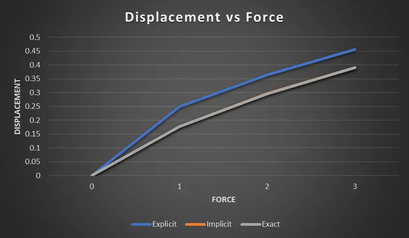
PLOT:
RESULT:
From the above plot the implicit and exact values are same and the explicit values diverge away from the exact values since there is no equilibrium between the internal and external forces. Thus implicit method is prefered for analysis.