Assignment 5-RADIOSS Interfaces & Study of Effect of Notches Challenge

AIM:

To study the RADIOSS Interfaces and the effect of notches using Hypermesh, Hyperview and Hypergraph 2D.

OBJECTIVES :

• To create mesh for bumper assembly, mesh element size is 6mm.
• To apply and study the different cases for the crash tube model.
• To study the effect of notches on the crash tube.
• To plot the Rwall forces, Internal energy and Contact energy graphs.
• To compare the case setups using the no of cycles, energy error, mass error, simulation time, and maximum von misses stress.
• To study the simulation animations.
• To conclude on the case results.

PROCEDURE:

MODEL 1 :

• First step is to import the model in Hypermesh.
• Go to FILE > IMPORT > MODEL > BROWSE > OPEN > IMPORT.

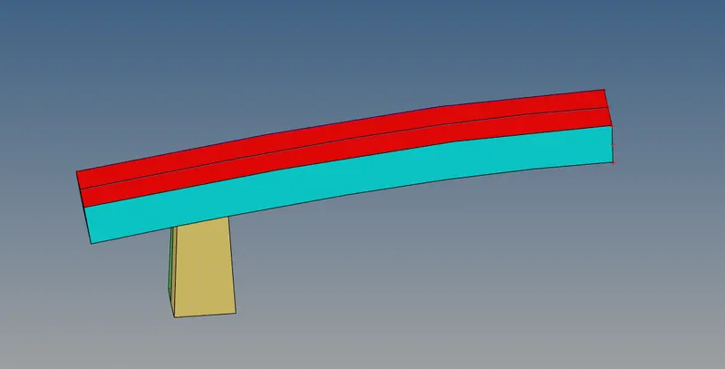
• This will import the model into Hypermesh software.
• Go to GEOM > TEMP NODES > CLEAR ALL to delete the temporary nodes.
• Go to GEOM >SURF EDIT > EXTEND > EXTEND OVER EDGES > SURFS: TO TARGET > EXTEND.

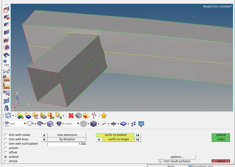
• This will extend the surfs to the next surface to make a T connection.

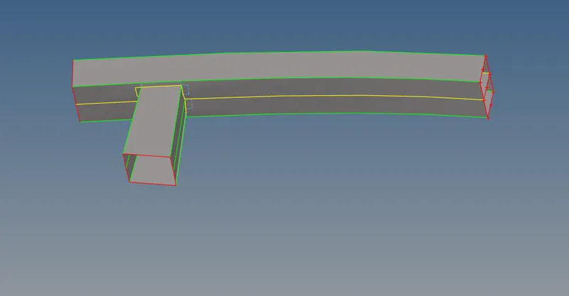
• Now, we have to deploy mesh for this model.
• Go to 2D > AUTOMESH > SURFS > DISPLAYED > ELEMENT SIZE = 6MM > ELEMENT TYPE = MIXED > MESH.

• This will deploy the mesh on the components.

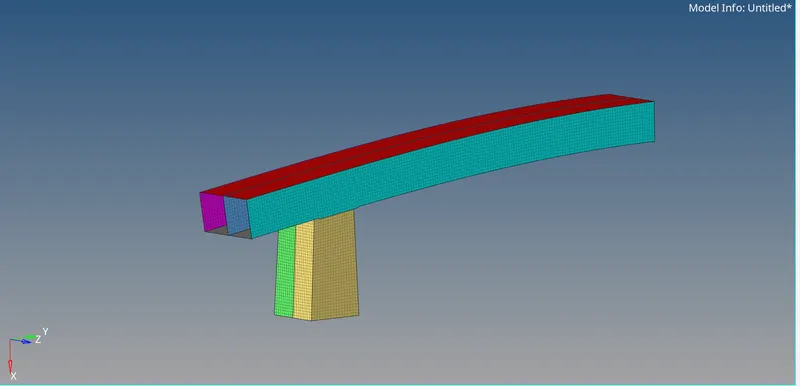
• Hence a mesh is created to the bumper system.

MODEL 2 :

Case 1: Run the crash tube model as it is.

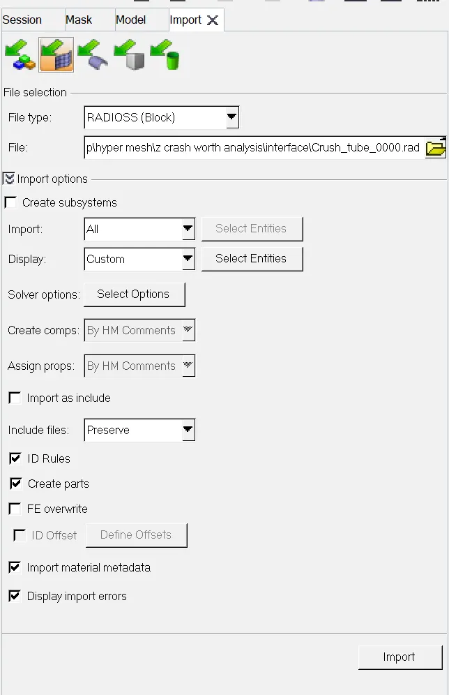
• Go to FILE > IMPORT > SOLVER DECK > CRUSH TUBE_0000.RAD > IMPORT.

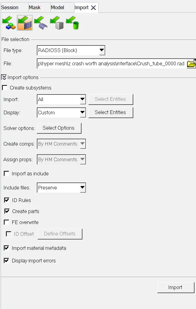
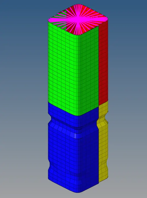
• For the first case we have to run the model as it is.
• Before running the file let’s have a look at the property card and the material card.

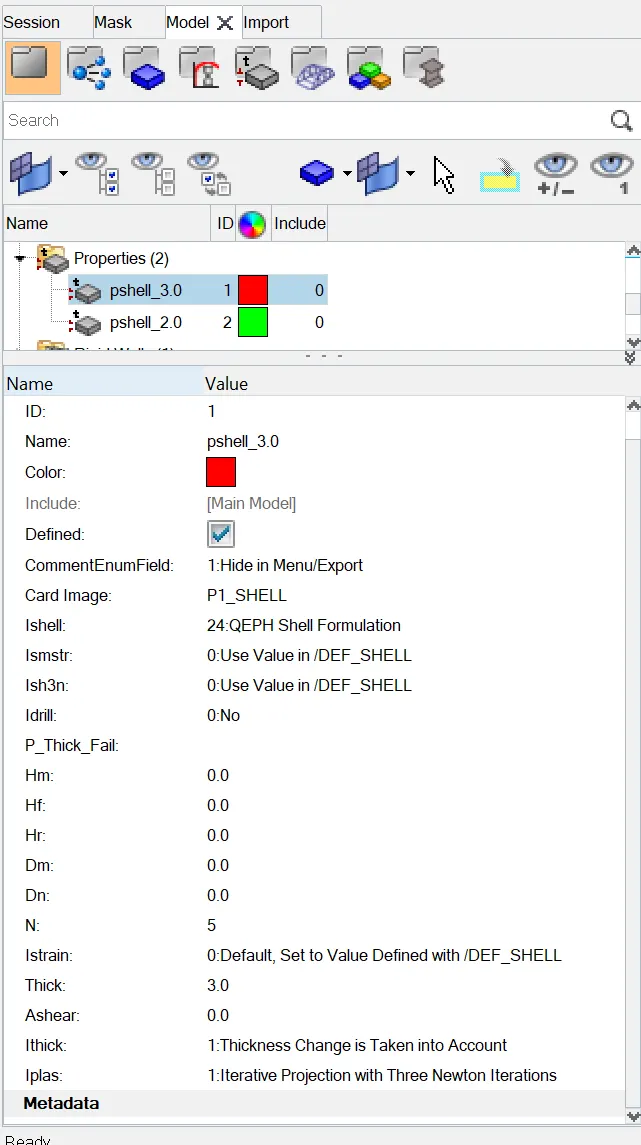
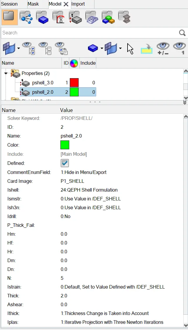
• Both the property card are set to the recommended property values.

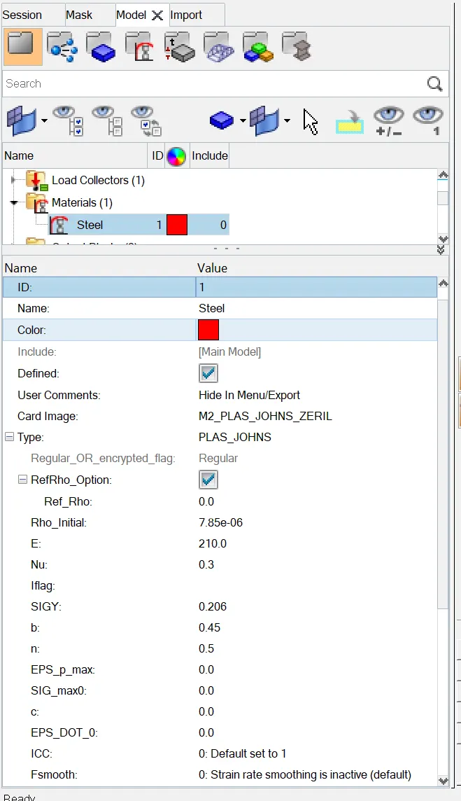
• The material card shows EPS_p_max value is zero.
• Now, go to ANALYSIS > RADIOSS > INPUT FILE > INCLUDE CONNECTOR > OPTIONS = -NT 4 > RADIOSS.

• This will run the Radioss simulation.
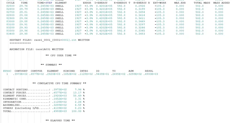
• Open .out engine file from saved folder and check final value of Energy error, Mass error, Simulation time and Total no of cycles.

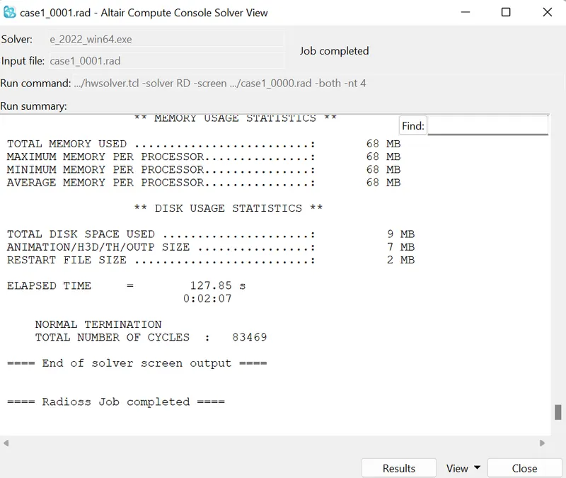
• Click on view Results, which will open Hyperview window.
• In Hyperview go to CONTOUR > RESULT TYPE > VON MISES > AVERAGING METHOD > SIMPLE > APPLY.

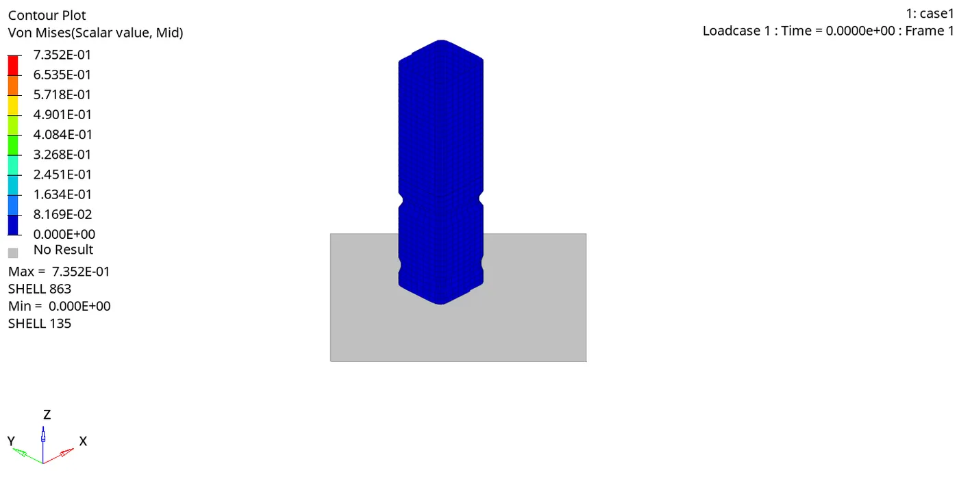
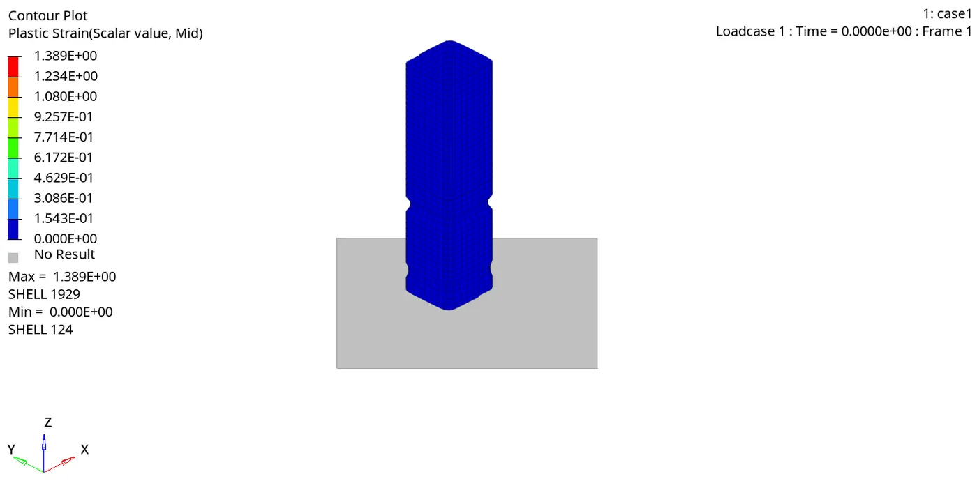
• In this simulation we can see that the tube starts to bend at the upper notch where the initial plastic strain occurs, and eventually the tube starts to bend at the lower notch. We can also observe that the tube fail between the notch region and then the region above the notch is crushed.
• The maximum Von misses stress and the maximum Plastic strain is formed at the corner section of the tube.
• Open Hypergraph 2D and load T01 file.
• Go to GLOBAL VARIABLES > INTERNAL ENEGRY, KINETIC ENERGY and TOTAL ENERGY > MAG > APPLY. This will plot the energy graph.

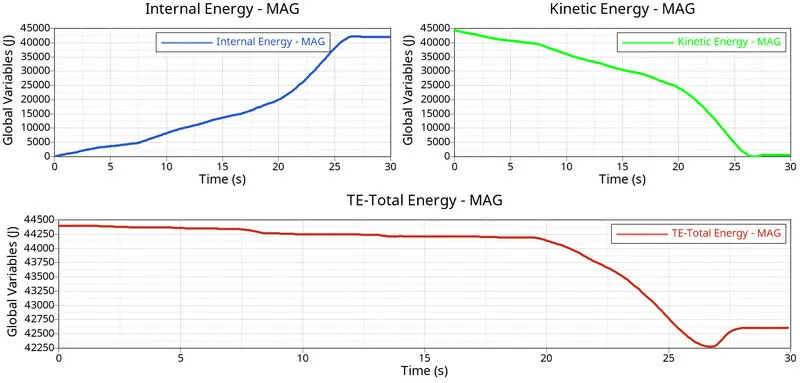
• The Kinetic energy having higher value at the start of the simulation eventually starts to reduce with time as it gets converted into Internal energy, because the can is being crushed. Thus, the total energy remains constant with respect to time, but we can see a slight drop in energy at time equals to 25ms. This is because the tube is totally crushed and the energy is lost to the friction between the elements.
• Go to GLOBAL VARIABLES > CONTACT ENERGY> MAG > APPLY. This will plot the energy graph.

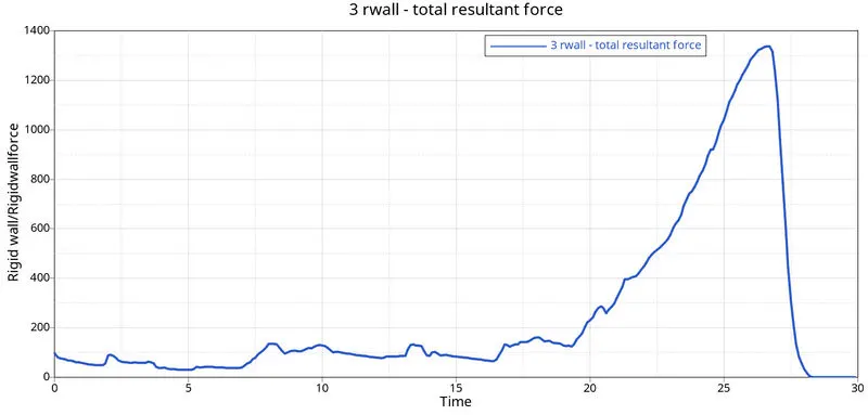
• The Kinetic energy having higher value at the start of the simulation eventually starts to reduce with time as it gets converted into Internal energy, because the can is being crushed. Thus, the total energy remains constant with respect to time, but we can see a slight drop in energy at time equals to 25ms. This is because the tube is totally crushed and the energy is lost to the friction between the elements.
• Go to GLOBAL VARIABLES > CONTACT ENERGY> MAG > APPLY. This will plot the energy graph.

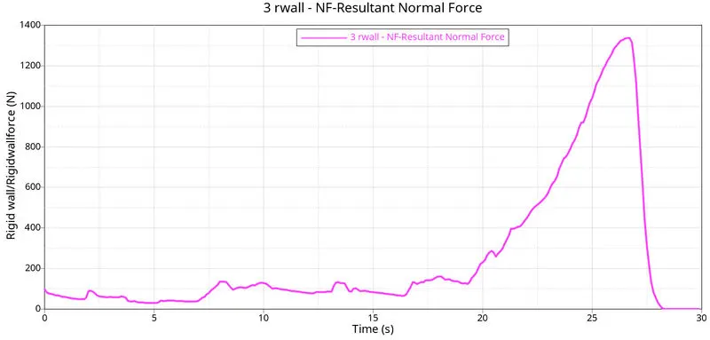
• A pattern is observed in the Resultant normal force, where a small amount of force increases at a regular interval of time. This increase in the force is when the corner edges fold the tube and the slave nodes try to penetrate into the master surface, the spring stiffness increase the force to oppose the slave node. After 20 ms we see a greater rise in the force value as the tube is crushed and more no of nodes come closer. Then the force is reduced and reaches to zero value.

Case 2: Change the Inacti=6 and run.

• Go to FILE > IMPORT > SOLVER DECK > CRUSH TUBE_0000.RAD > IMPORT.
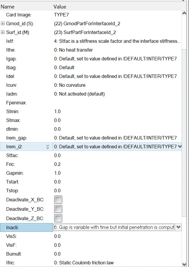
• Go to INTER > TYPE 7 > INACTI = 6.

• Now, go to ANALYSIS > RADIOSS > INPUT FILE > INCLUDE CONNECTOR > OPTIONS = -NT 4 > RADIOSS.
• This will run the Radioss simulation.

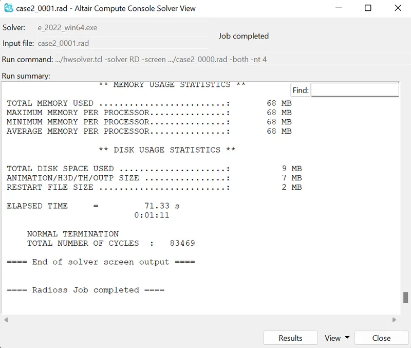
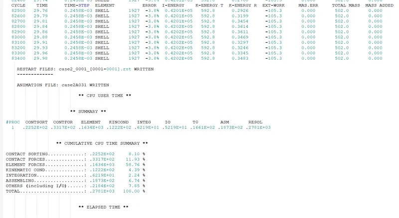
• Open .out engine file from saved folder and check final value of Energy error, Mass error, Simulation time and Total no of cycles.

• Click on view Results, which will open Hyperview window.
• In Hyperview go to CONTOUR > RESULT TYPE > VON MISES > AVERAGING METHOD > SIMPLE > APPLY.

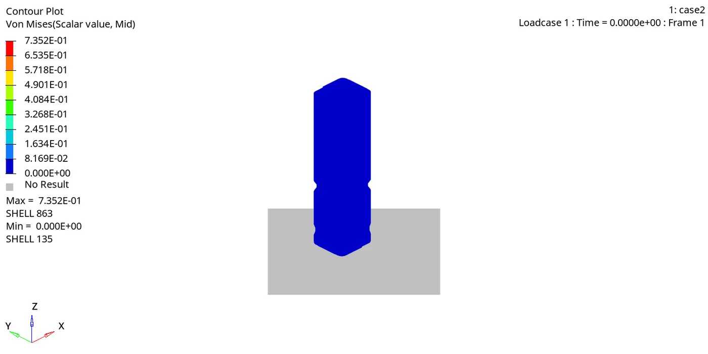
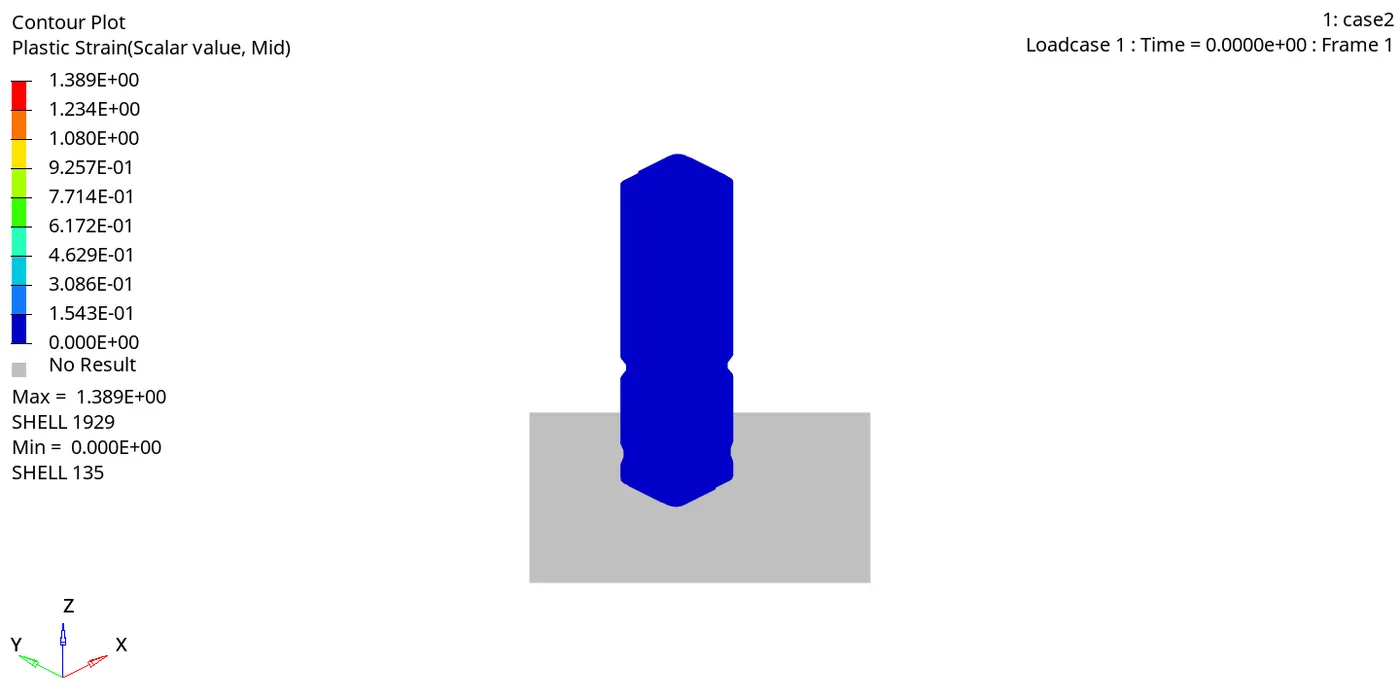
• The simulation is same as the case 1 simulation. There is no Geometric change in the model and also in the maximum stress and the strain values.
• The only change in this case is that Inacti6 is set, which reduces the gap and uses the scaling.
• Inacti6 removes the initial penetration and moves nodes 30% of the initial gap to avoid contact stability issues. As this is performed before the simulation, we observe no difference in the simulation as in case 1.
• Open Hypergraph 2D and load T01 file.
• Go to GLOBAL VARIABLES > INTERNAL ENEGRY, KINETIC ENERGY and TOTAL ENERGY > MAG > APPLY. This will plot the energy graph.

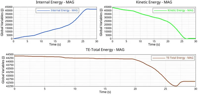
• The energy graph is same as the case 1.
• Go to GLOBAL VARIABLES > CONTACT ENERGY> MAG > APPLY. This will plot the energy graph.

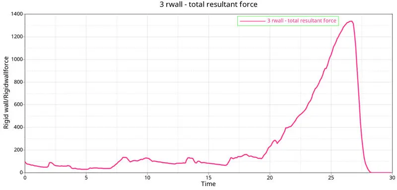
• The contact energy increases when the friction contact is defined. At 20 ms the contact energy increases due to the friction formulation defined.
• Go to GLOBAL VARIABLES > RWALL > NORMAL RESULTANT, TANGENT AND TOTAL FORCES > APPLY. This will plot the rigid wall forces.

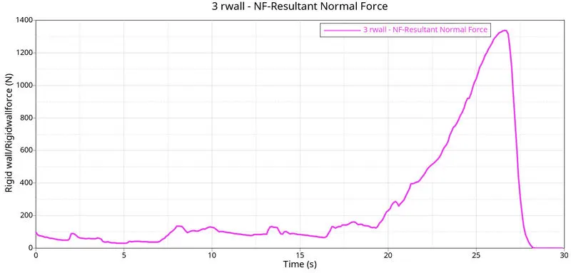
• The force graph is similar to the earlier case. The resultant normal force and total resultant force is similar as the variation in resultant tangent force is negligible.

Case 3: Create the type 11 contact and run.

• Go to FILE > IMPORT > SOLVER DECK > CRUSH TUBE_0000.RAD > IMPORT.
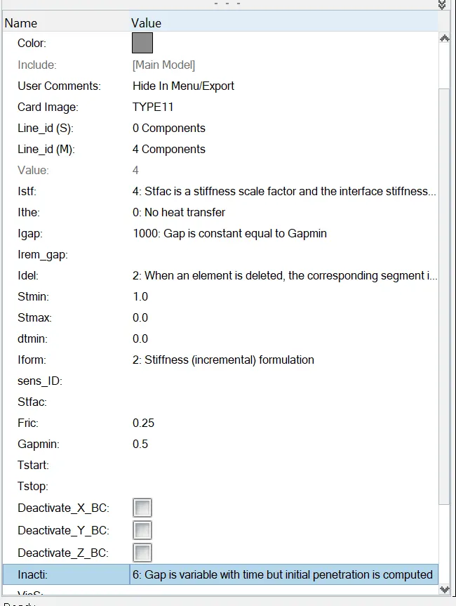
• CREATE > INTERFACE > TYPE 11 and set the following values in the card as shown in the image. Select all the 4 components for the master and slave line.

• Now, go to ANALYSIS > RADIOSS > INPUT FILE > INCLUDE CONNECTOR > OPTIONS = -NT 4 > RADIOSS.

• This will run the Radioss simulation.

• Open .out engine file from saved folder and check final value of Energy error, Mass error, Simulation time and Total no of cycles.

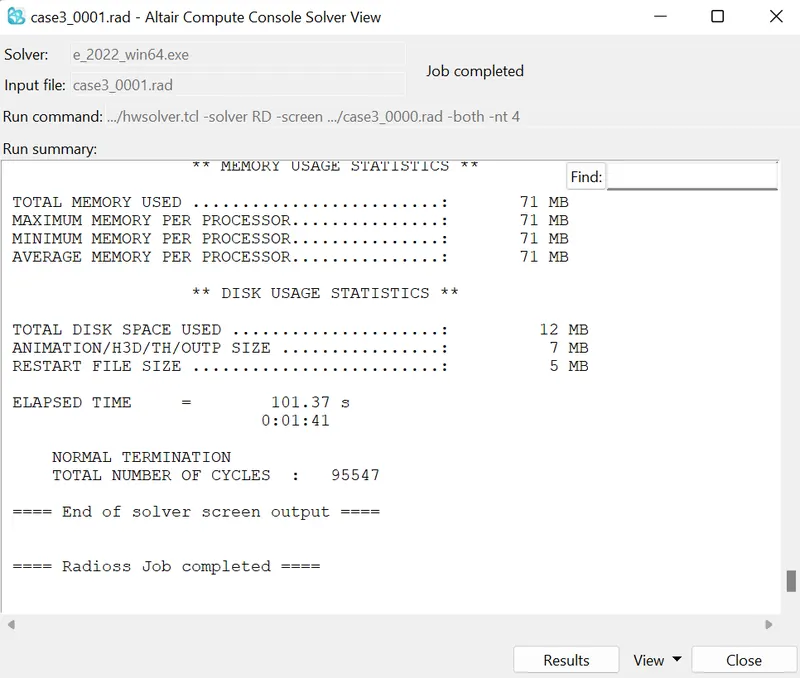
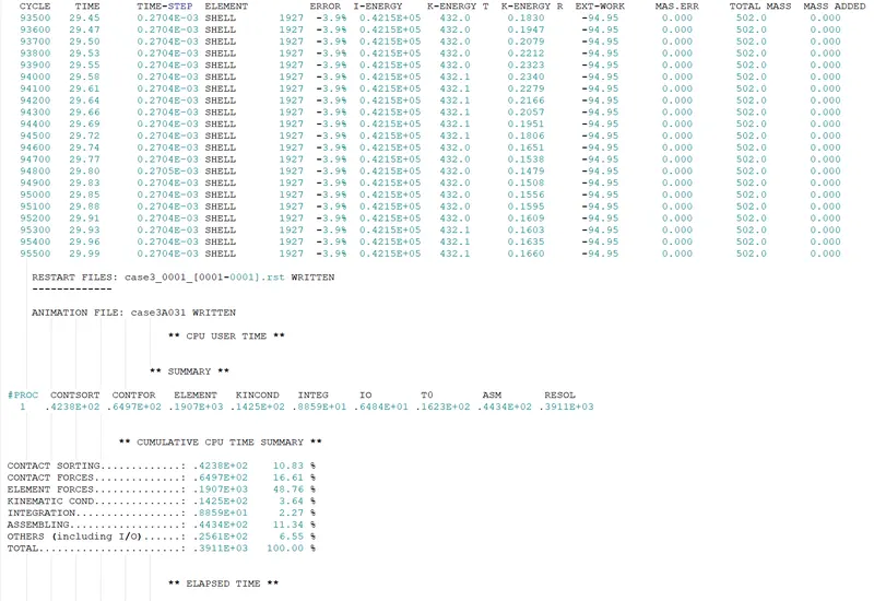
• Click on view Results, which will open Hyperview window.
• In Hyperview go to CONTOUR > RESULT TYPE > VON MISES > AVERAGING METHOD > SIMPLE > APPLY.

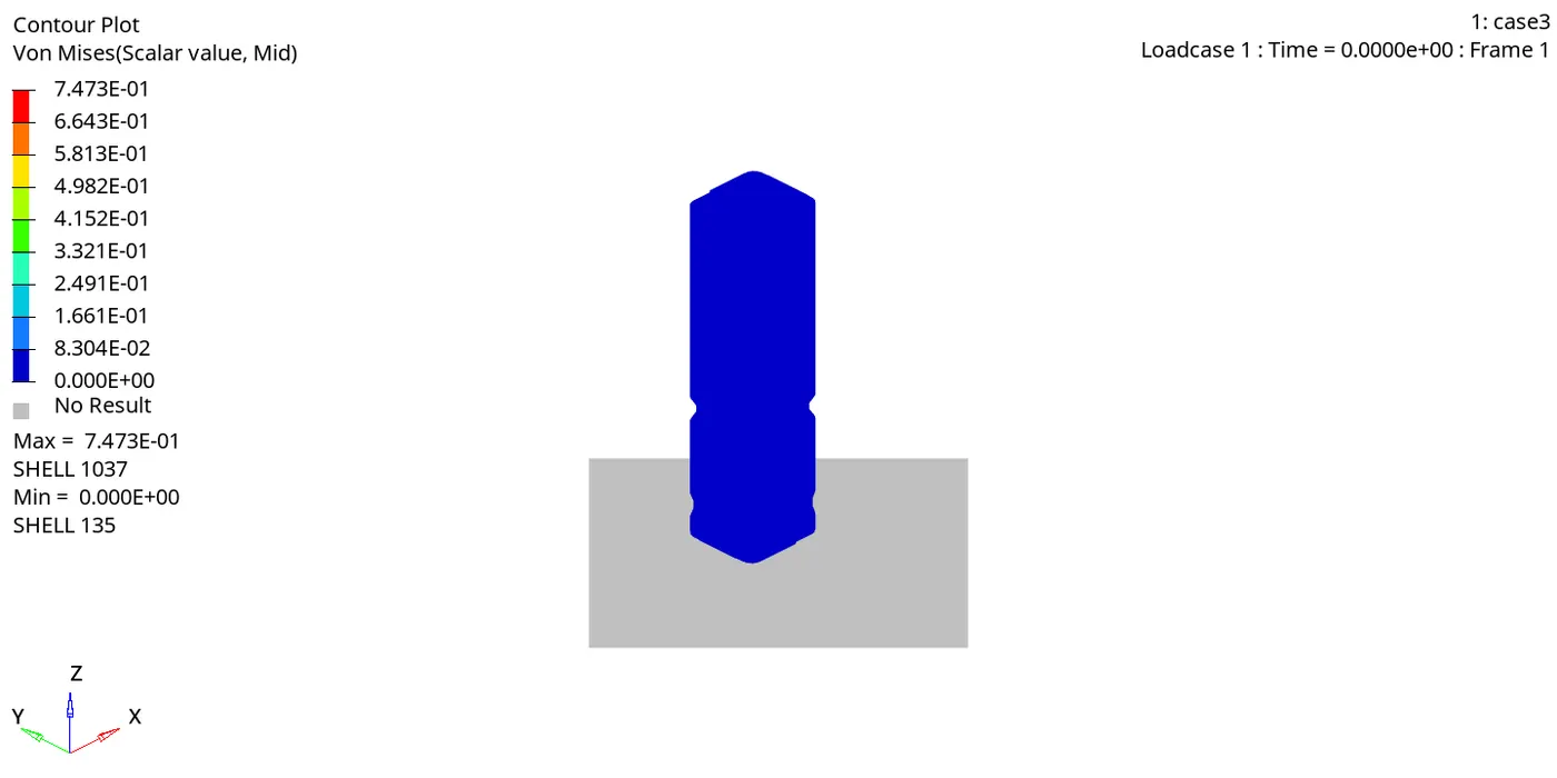
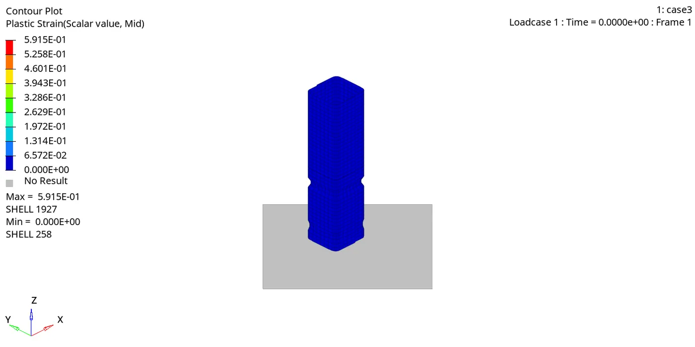
• In this case Type 11 interface is used which removes the edge to edge intersections. In the model as there are few edges the result doesnt vary with respect to the earlier results.
• Open Hypergraph 2D and load T01 file.
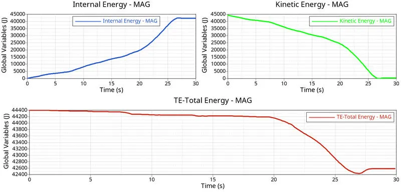
• Go to GLOBAL VARIABLES > INTERNAL ENEGRY, KINETIC ENERGY and TOTAL ENERGY > MAG > APPLY. This will plot the energy graph.

• Go to GLOBAL VARIABLES > CONTACT ENERGY> MAG > APPLY. This will plot the energy graph.

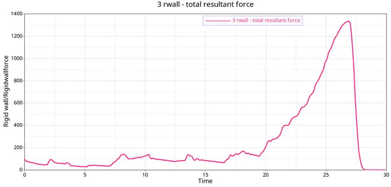
• Go to GLOBAL VARIABLES > RWALL > NORMAL RESULTANT, TANGENT AND TOTAL FORCES > APPLY. This will plot the rigid wall forces.

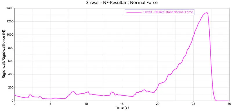
• The graphs are similar as discussed earlier.
• There is more energy error than type 7 interface.

Case 4: Remove both notches and remove boundary condition on rigid body node then run.

• Go to FILE > IMPORT > SOLVER DECK > CRUSH TUBE_0000.RAD > IMPORT.
• For this case we have to remove the notches and delete the boundary condition.
• Press F7 to go to the node edit panel. Align the nodes with the align option in the nodes-edit panel.

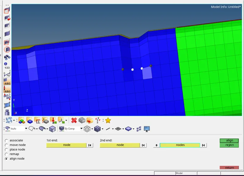
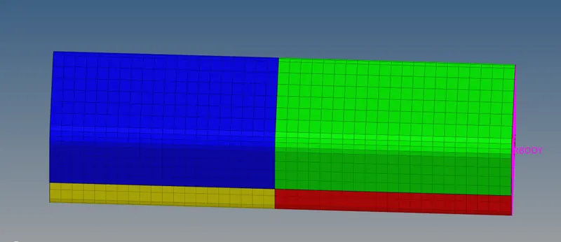
The notches were removed.

• Go to the BOUNDARY CONDITIONS > DELETE, to delete the boundary conditions.

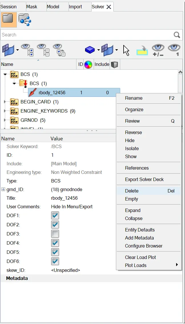
• Now, go to ANALYSIS > RADIOSS > INPUT FILE > INCLUDE CONNECTOR > OPTIONS = -NT 4 > RADIOSS.
• This will run the Radioss simulation.

• Open .out engine file from saved folder and check final value of Energy error, Mass error, Simulation time and Total no of cycles.

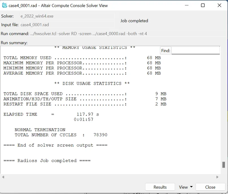
• Click on view Results, which will open Hyperview window.
• In Hyperview go to CONTOUR > RESULT TYPE > VON MISES > AVERAGING METHOD > SIMPLE > APPLY.

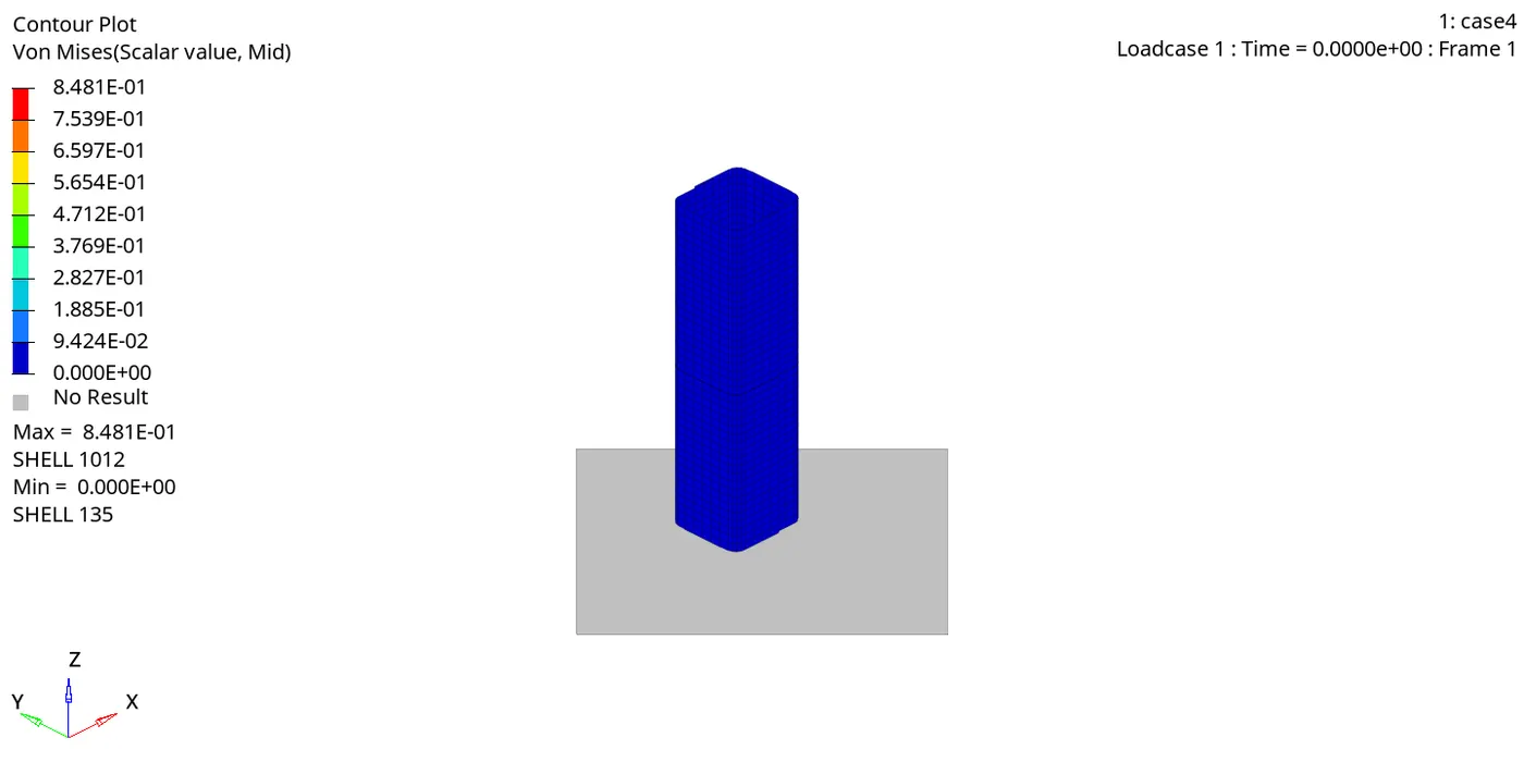
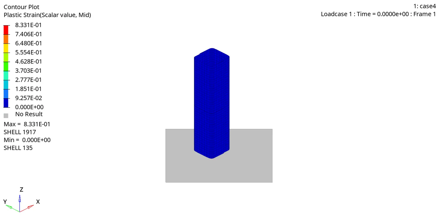
• In this case, the notches are removed and hence we have a uniform section. The tube starts deforming at the bottom region and the same layered pattern is followed for deformation. The maximum von misses stress measured is a bit less than the earlier cases.
• Open Hypergraph 2D and load T01 file.
• Go to GLOBAL VARIABLES > INTERNAL ENEGRY, KINETIC ENERGY and TOTAL ENERGY > MAG > APPLY. This will plot the energy graph.

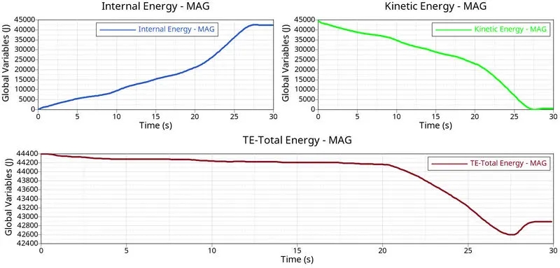
• Due to notch removal the drop in the kinetic energy at the end in not seen. Hence, the total energy remains almost constant.
• Go to GLOBAL VARIABLES > CONTACT ENERGY> MAG > APPLY. This will plot the energy graph.

• The contact energy is lower than 1300 kgmm2/ms2, where previously the contact energy increased above 1350 kgmm2/ms2. This reduction is due to less friction between the elements as the notch is removed.

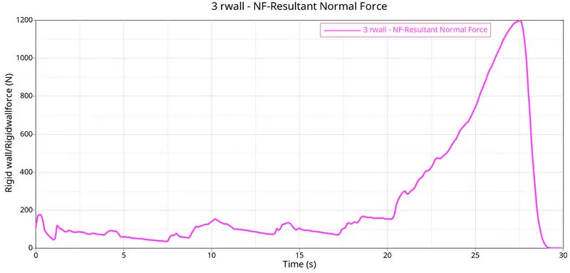
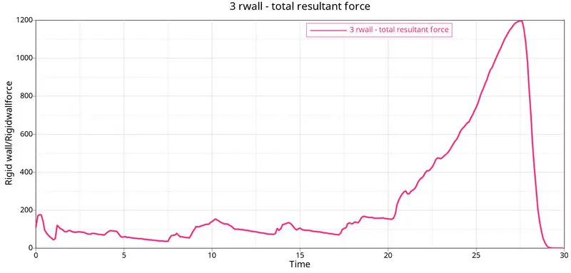
• The resultant normal and the total resultant force is observed to be less than the previous cases. The max force value is 1200 KN where the previous cases recorded upto 1350 KN.
• This drop is due to the removal of the Boundary condition.

Case 5: Create a new notch in the middle ,select the whole section and run.

• Go to FILE > IMPORT > SOLVER DECK > CRUSH TUBE_0000.RAD > IMPORT.
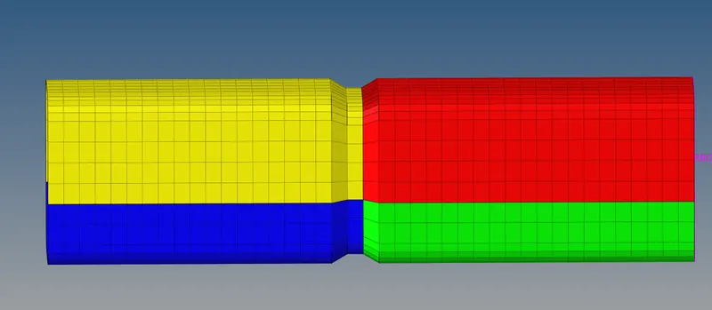
• For this case we have to create a notch at the middle section.
• Hence, first use align option for removing all the notches and then go to TOOL > TRANSLATE option to create a notch at the middle section.

• Now, go to ANALYSIS > RADIOSS > INPUT FILE > INCLUDE CONNECTOR > OPTIONS = -NT 4 > RADIOSS.

• This will run the Radioss simulation.

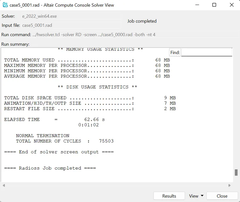
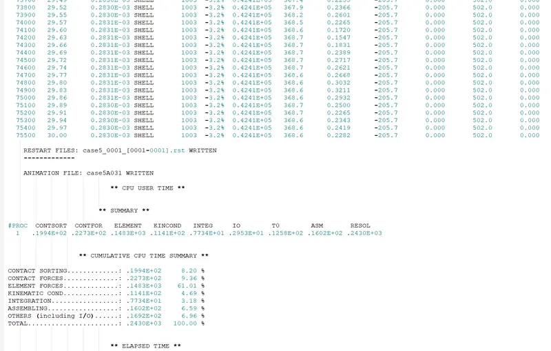
• Open .out engine file from saved folder and check final value of Energy error, Mass error, Simulation time and Total no of cycles.

• Click on view Results, which will open Hyperview window.
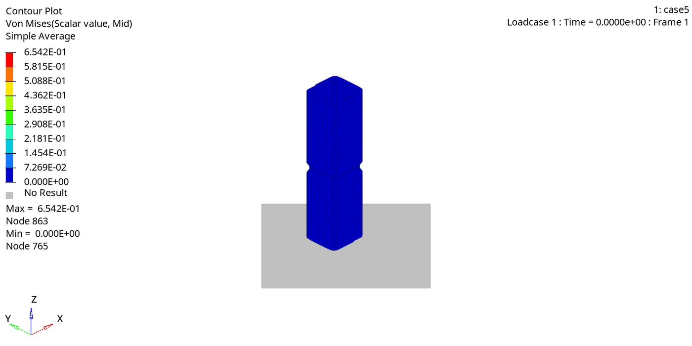
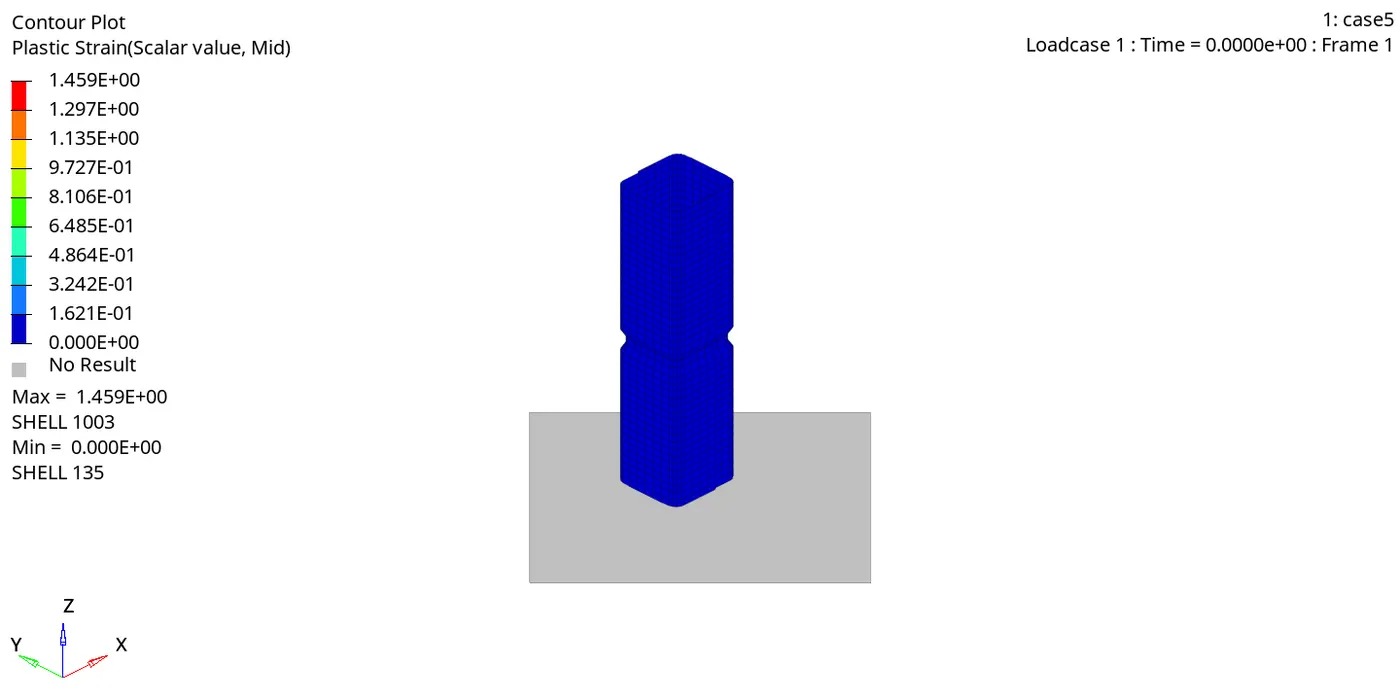
• In Hyperview go to CONTOUR > RESULT TYPE > VON MISES > AVERAGING METHOD > SIMPLE > APPLY.

• Open Hypergraph 2D and load T01 file.
• Go to GLOBAL VARIABLES > INTERNAL ENEGRY, KINETIC ENERGY and TOTAL ENERGY > MAG > APPLY. This will plot the energy graph.

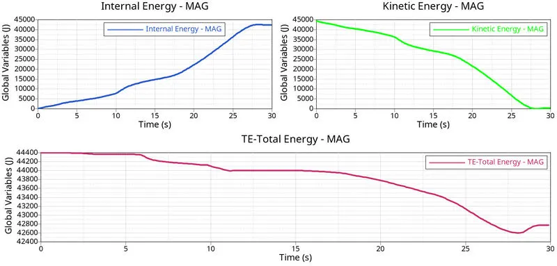
• In this graph we can observe a slight reduction in teh kinetic energy and a slight increase in the internal energy at 11ms, where the deformation in the upper section starts. This is mainly due to the notch created at the middle section of the tube.
• Go to GLOBAL VARIABLES > CONTACT ENERGY> MAG > APPLY. This will plot the energy graph.

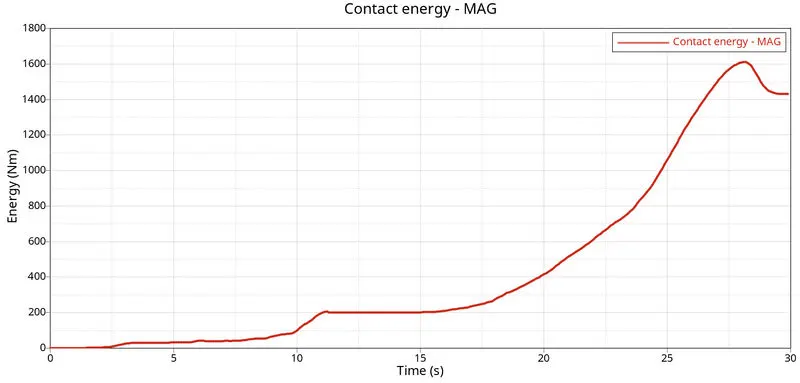
• Here we can see that the contact energy slightly increases at the point of shift of deformation. Also the contact energy at the end is above 1500 kgmm2/ms2.

• Go to GLOBAL VARIABLES > RWALL > NORMAL RESULTANT>APPLY.
• This will plot the rigid wall forces.

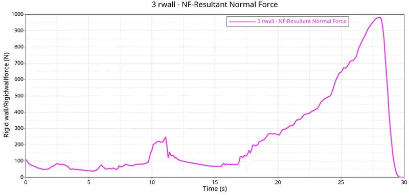
• In the previous cases we observed a slight increase in the forces where the deformation shifted from the notch sections. Similarly, a single(as we have only one notch) slight rise and fall in the forces is seen at 11ms where the deformation is shifted to the upper section of the tube.

Case 6: Create a new notch with nodes only from opposing 2 faces and run.

• Go to FILE > IMPORT > SOLVER DECK > CRUSH TUBE_0000.RAD > IMPORT.
• For this case we have to create a notch with nodes only from opposite two faces.
• Hence, first use align option for removing all the notches and then go to TOOL > TRANSLATE option to create a notch on the opposite two faces.

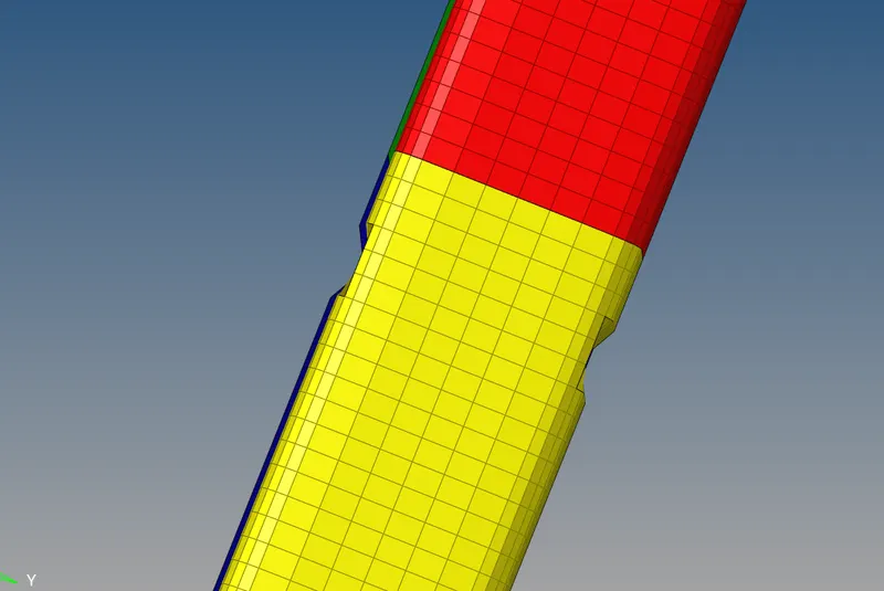
• Now, go to ANALYSIS > RADIOSS > INPUT FILE > INCLUDE CONNECTOR > OPTIONS = -NT 4 > RADIOSS.

• This will run the Radioss simulation.
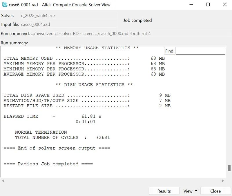
• Open .out engine file from saved folder and check final value of Energy error, Mass error, Simulation time and Total no of cycles.

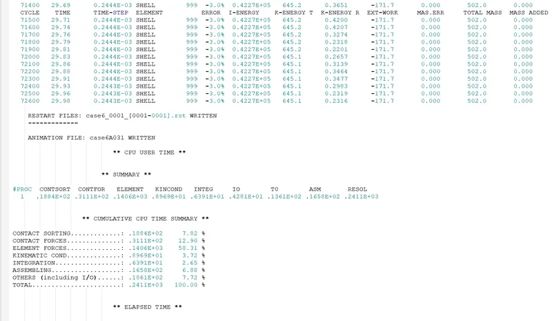
• Click on view Results, which will open Hyperview window.
• In Hyperview go to CONTOUR > RESULT TYPE > VON MISES > AVERAGING METHOD > SIMPLE > APPLY.

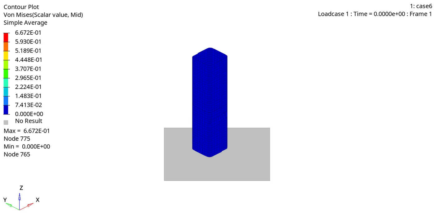
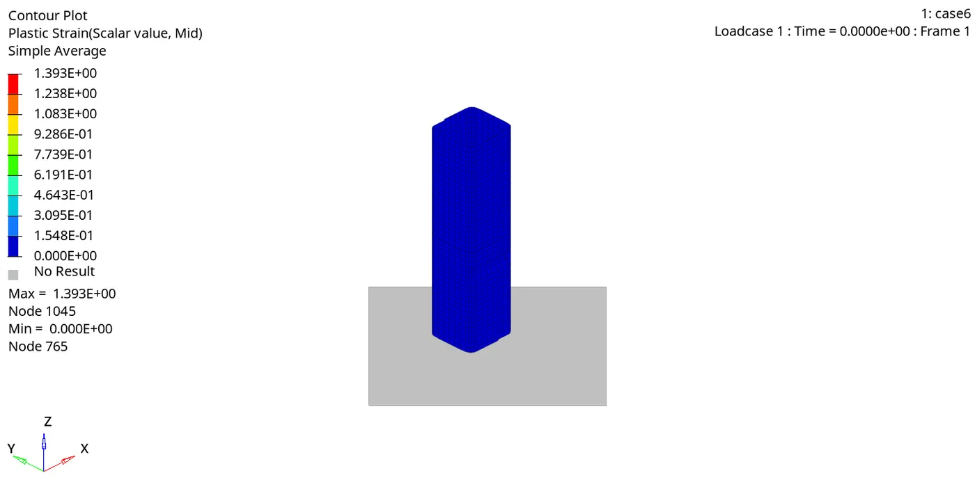
• In this case the initial deformation is again at the notch section due to the stress concentration. But the faces having the notch deform inwards and the faces with no notch deform outward.
• Open Hypergraph 2D and load T01 file.
• Go to GLOBAL VARIABLES > INTERNAL ENEGRY, KINETIC ENERGY and TOTAL ENERGY > MAG > APPLY. This will plot the energy graph.

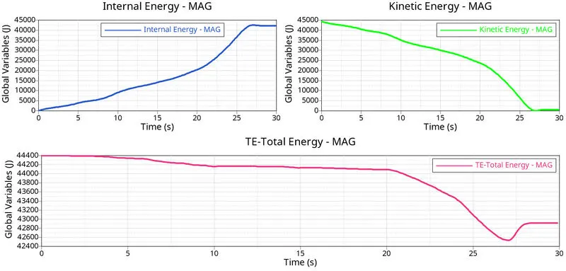
• As compared to the previous cases the graph does not show slight deformation at 11ms.
• Go to GLOBAL VARIABLES > CONTACT ENERGY> MAG > APPLY. This will plot the energy graph.

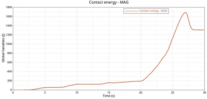
• The contact energy recorded is lower than the previous cases. The contact energy at the end is about 1500 kgmm2/ms2. The increase in the contact energy at the beginning is very less.
• Go to GLOBAL VARIABLES > RWALL > NORMAL RESULTANT > APPLY. This will plot the rigid wall forces.

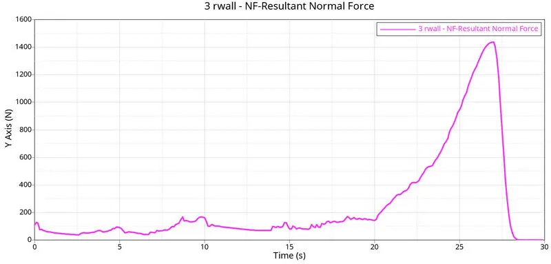
The resultant Normal force shows ups and downs also at the peak region.

RESULTS:

Case No	Total no of cycles	Energy Error	Mass Error	Simulation Time (sec)	Max Von Mises Stress
1	83469	-3.8%	0	121.85	0.7352
2	83469	-3.8%	0	71.33	0.7352
3	95547	-3.9%	0	101.37	0.7473
4	78390	-3.0%	0	117.97	0.8481
5	75503	-3.2%	0	62.66	0.6542
6	72681	-3.0%	0	61.81	0.6672

• In Case 1 energy error is -3.8% and mass error 0%. The simulation time 121.85 Sec.
• Here type 7 interface is used for the first two cases and then the type 11 contact is created. Hence. both the interface work together making the simulation stable. The deformation of the tube is observed to be in layers, where the slave nodes try to enter the master gap, the penalty method creates a spring and resistive forces are applied.
• In the second case, we only observe the change in simulation time, because the Inacti6 is set which performs initial penetration checks before the simulation.
• In the third case the type 7 and type 11 interface work together increasing the simulation time. The energy error is also increased.
• In the fourth case. we observe less no of cycles and lower energy error as the boundary conditions and the notches are removed.
• In the fifth case, we observe the increase in the energy error due to the notch created at the middle section here the four components are closer to each other when deformed.
• In sixth case, we observe the no of cycles to be the greatest among all the cases. Also there is reduction in the energy error as opposite face notch is created.

LEARNING OUTCOMES:

• To apply the different interfaces for the components.
• To study the results of the interface types.
• To understand the parameter checks before simulation and during simulation.
• The significance of Inacti 6.
• To plot the energy and the rigid wall forces.

CONCLUSION:

• The given bumper model in meshed.
• Hence, by performing this project we conclude that the we have studied the type 7 and type 11 interface and also their working together. We also studied the effect of notches based upon their location and no of notches. The parameters checked before the simulation and during the simulation are also studied.