Week - 8 Mass Scaling

AIM:

    To introduce mass scaling Technique to reduce the run time for the analysis and the limit for the mass scaling is restricted to 8% and simulation as to be completely stable. By optimizing the TSSFC and DT2MS parameters the simulation is analyzed.

INTRODUCTION:

Timestep Significance:

In the simplest case (small, deformation theory), the time step is controlled by the acoustic wave propagation through the material

In explicit integration, the numerical stress wave must always propagate less than one element width per time step. The time step of an explicit analysis is determined as the minimum stable time step in any one deformable finite element in the mesh. The above relationship is called the Courant-Friedrichs-Lewy (CFL) condition and determines the stable time step in an element. 

The CFL condition requires that the explicit time step be smaller than the time needed by the physical wave to cross the element. 0.9 is the timestep scale factor (TSSFAC). Based on the conditions, the time step can be increased to provide faster solution times by artificially increasing the density of the material by using a technique  like ( mass scaling, lowering the modulus, or by increasing the element size of the mesh)

2) Mass scaling:

Mass-scaling is a term that is used for the process of scaling the element’s mass in explicit simulations to adjust its timestep. The primary motivation is to change (usually increase) the global compute timestep which is limited by the Courant’s stability criteria Mass scaling is very useful and directly increases the timestep. The concept is simple, Larger Timestep = Lower Solution Time. The manual form of mass scaling is done independently of the automatic mass scaling invoked with DT2MS in *CONTROL_TIMESTEP.

*CONTROL_TIMESTEP: Conventional mass scaling (CMS) (negative value of DT2MS): The mass of small or stiff elements is increased to prevent a very small timestep. Thus, artificial inertia forces are added which influence all eigenfrequencies including rigid body modes. This means this additional mass must be used very carefully so that the resulting nonphysical inertia effects do not dominate the global solution. 

 Two different types of mass-scaling using the DT2MS parameter from *CONTROL_TIMESTEP

• Negative DT2MS: Mass is added to only those elements whose timestep would otherwise be less than TSSF*(DT2MS). When mass scaling is appropriate.
• Positive DT2MS: Mass is added or taken away from elements so that the timestep of every element is the same.  there is no advantage to using this method over the negative DT2MS method and I find it harder to rationalize.

If stability is a problem with the default TSSFAC of 0.9, try 0.8 or 0.7. If you reduce TSSFAC, you can increase |DT2MS| proportionally so that their product, and hence timestep, is unchanged. TSSFAC doesn’t affect the mass scaling percentage.

Mass scaling is no free lunch. For dynamic systems, added mass can affect the response of the system. It is just something to monitor and make an engineering judgment about its effectiveness; time savings versus potential detrimental effects. Increasing the mass too much may cause severe penetration problems and increase the dynamic effect significantly. The results may not be acceptable. In this case, the mass scaling is restricted up to 8%.

PROCEDURE:

        The DTMS and TSSFAC are the important parameters in the  *CONTROL_TIMESTEP card that affects the timestep and the runtime of the simulation, so we will change these values in each iteration to obtain an optimized runtime with a stable solution and to make sure mass scaling doesn’t go beyond 8%.

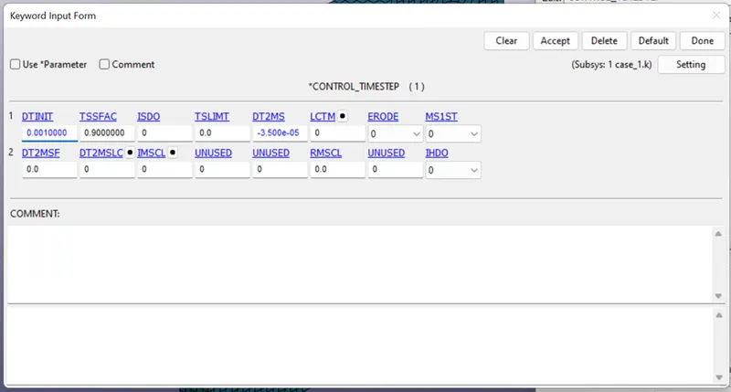
Case-1: DT2MS: -3.5E-5 & TSSFAC: 0.9

In the first case, we set the *CONTROL_TIMESTEP card parameters to default values as shown in the image given below.

We run the simulation and get the following output as shown in the image given below.

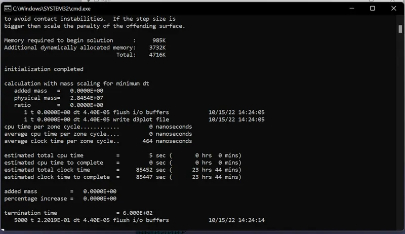
We get the estimated time: 23 hrs 44 mins and the added mass: 0.

Case-2: DT2MS: -3.0E-5 & TSSFAC: 0.9

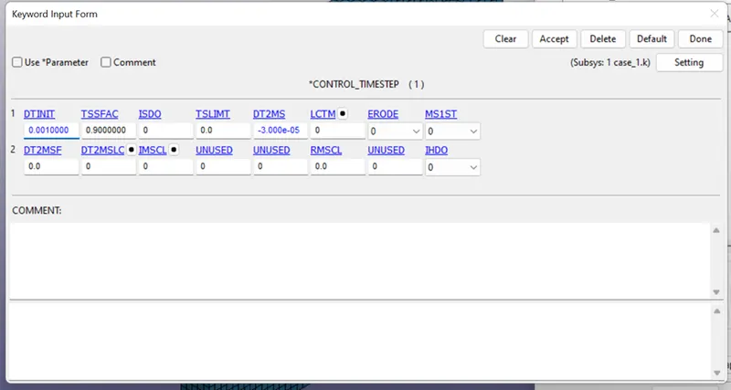
We run the simulation and get the following output as shown in the image given below.

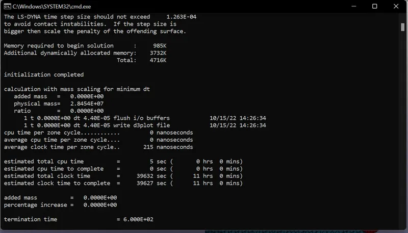
We get the estimated time: 11 hrs 0 mins and the added mass: 0.

Case-3: DT2MS: -2E-5 & TSSFAC: 0.9

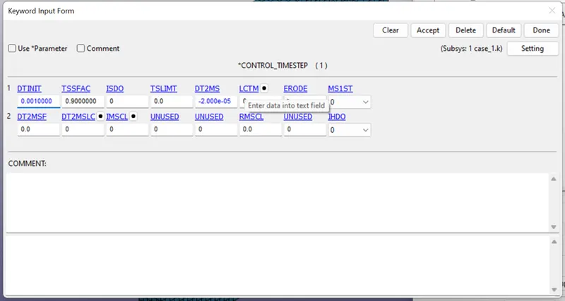
We run the simulation and get the following output as shown in the image given below.

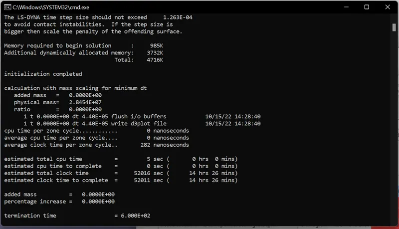
We get the estimated time: 14 hrs 26 mins and the added mass: 0.

Case-4: DT2MS: -1E-5 & TSSFAC: 0.9

.

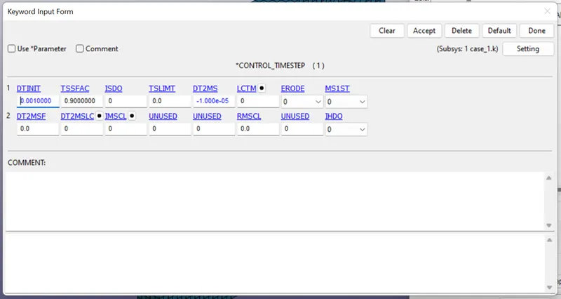
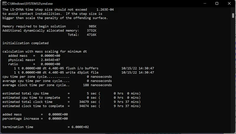
Case-5: DT2MS: -3.0E-4 & TSSFAC: 0.9

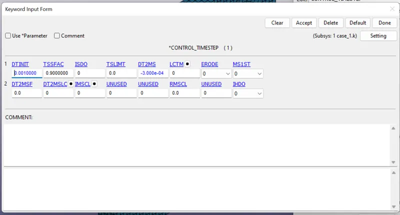
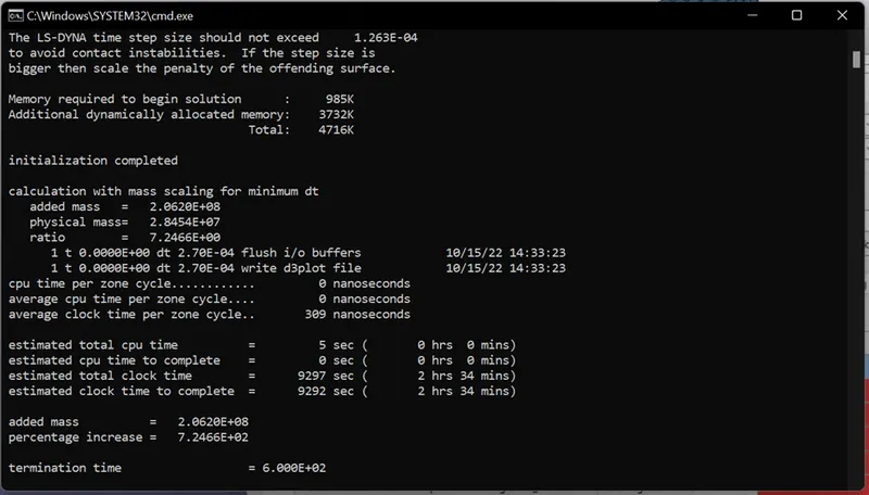
We get the estimated time: 2 hrs 34 mins and the added mass:7.24 %

Case-6: DT2MS: -2E-4 & TSSFAC: 0.9

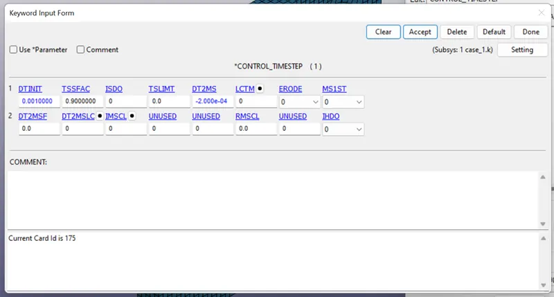
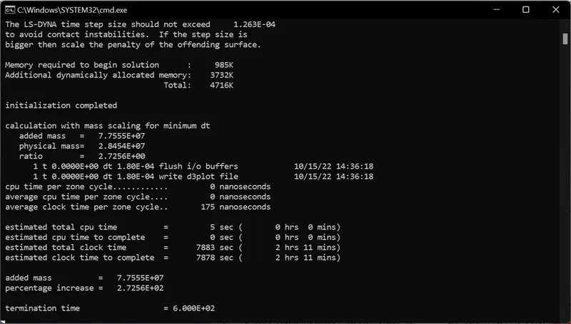
We get the estimated time: 2 hrs 11 mins and the added mass: 2.72 %.

Case-7: DT2MS: -1E-4 & TSSFAC: 0.9

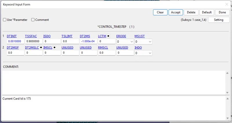
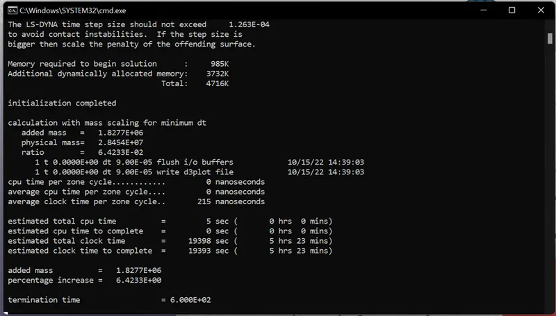
We get the estimated time: 5 hrs 23 mins and the added mass:6.42 %

 Case-8: DT2MS: -1.05E-4 & TSSFAC: 0.9

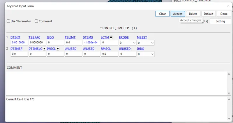
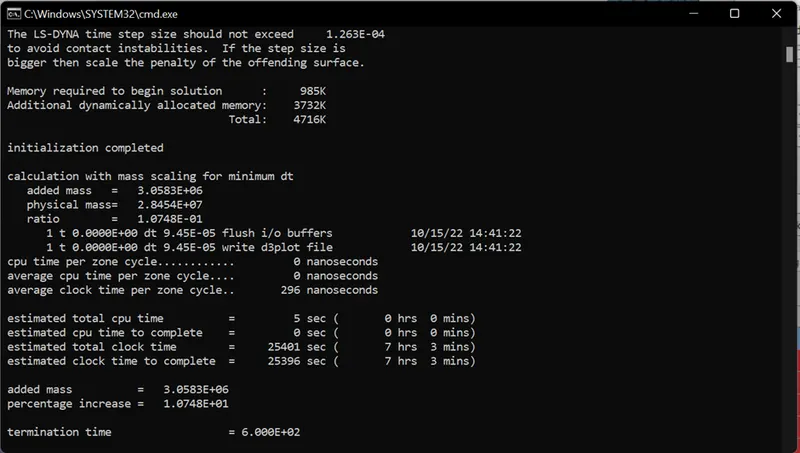
We get the estimated time: 7 hrs 03 mins and the added mass: 10.748 % which is more than 8% which is not acceptable. So the scale of decreasing value of DT2MS should be less.

Case-9: DT2MS: -1.03E-4 & TSSFAC: 0.9

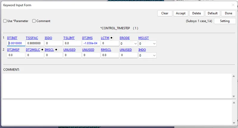
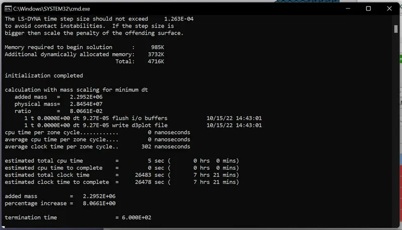
We get the estimated time: 7 hrs 21 mins and the added mass: 8.066 %

Case-10: DT2MS: -1.029E-4 & TSSFAC: 0.9

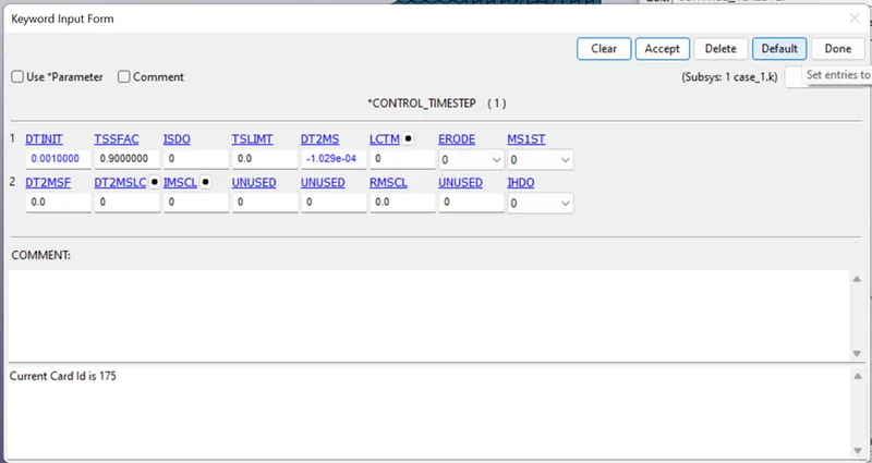
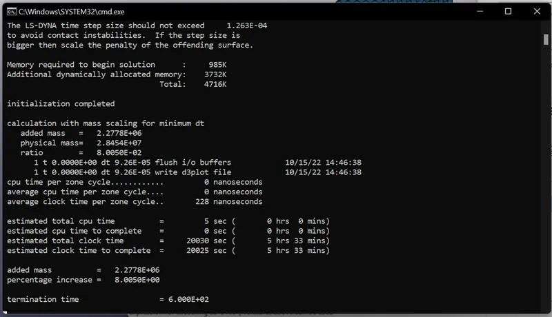
We get the estimated time: 5 hrs 33 mins and the added mass: 8.005 %

Case-11: DT2MS: -1.029E-4 & TSSFAC: 0.8

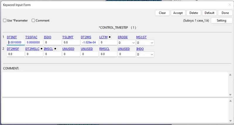
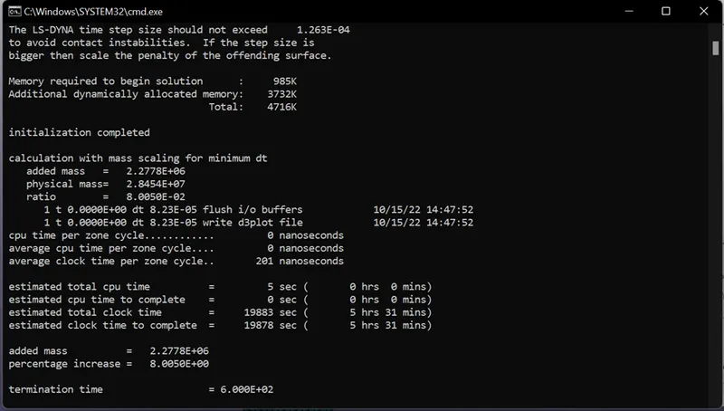
We get the estimated time: 5 hrs 31 mins and the added mass: 8.005 %

Case-12: DT2MS: -1.029E-4 & TSSFAC: 0.7

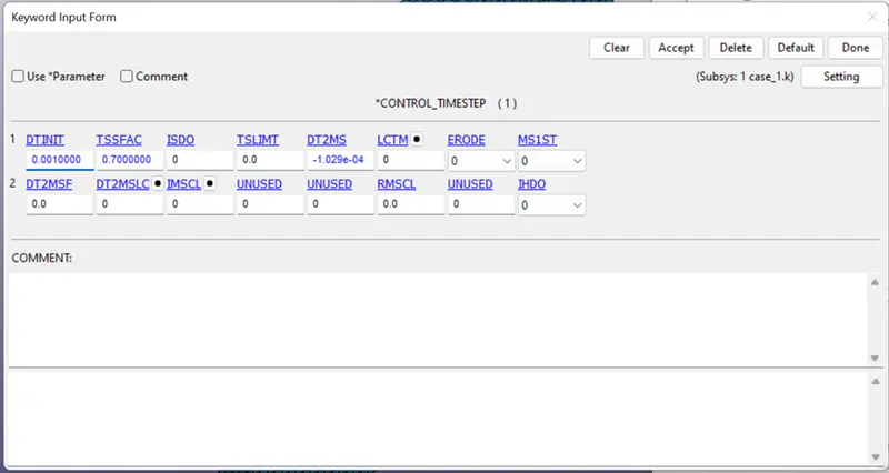
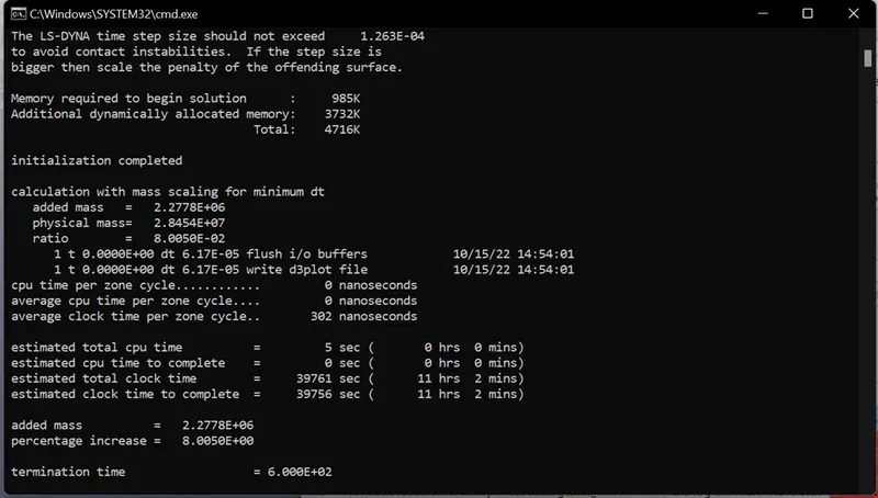
We get the estimated time: 11 hrs 02 mins and the added mass: 8.005 %

 Case-13: DT2MS: -1.029E-4 & TSSFAC: 0.6

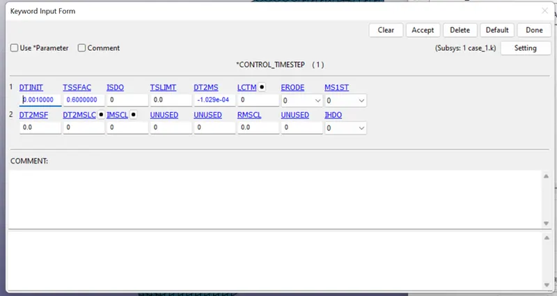
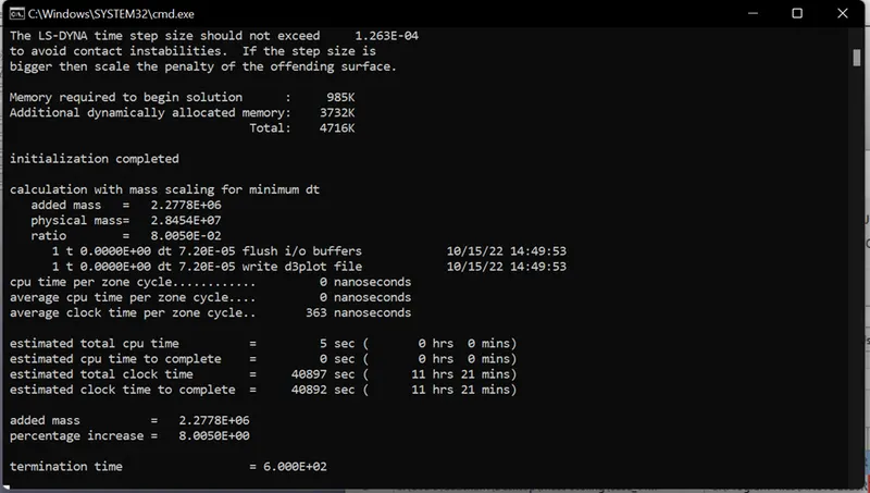
We get the estimated time: 11 hrs 21 mins and the added mass: 8.005 %

Case-14: DT2MS: -1.029E-4 & TSSFAC: 0.5

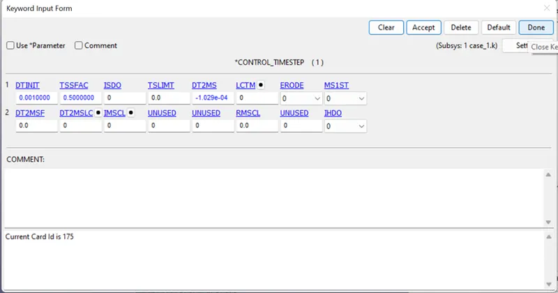
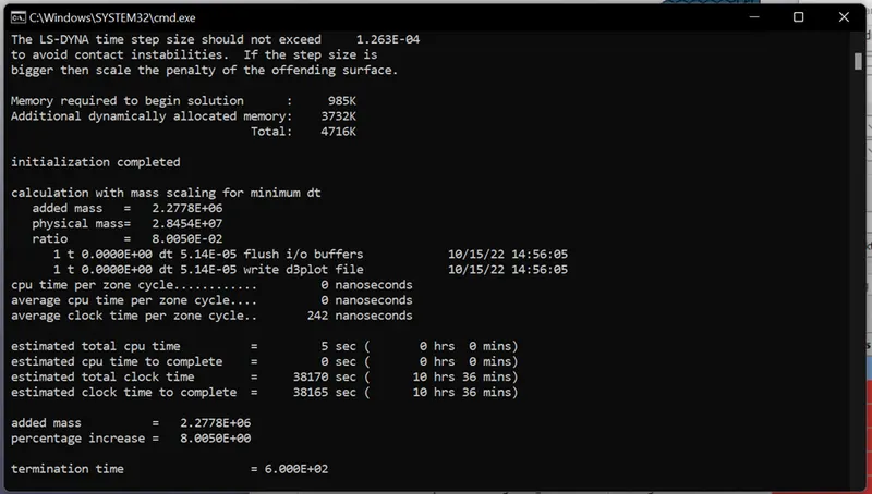
We get the estimated time: 10 hrs 36 mins and the added mass: 8.005 % 

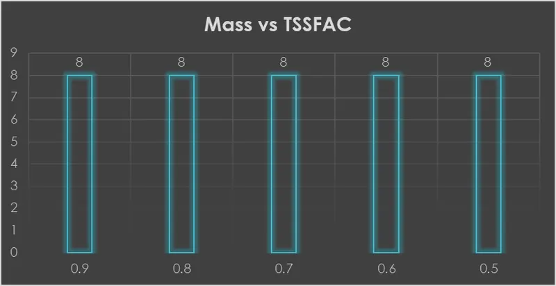
     We see that the time scale factor doesn't change the amount or percentage of mass added as the mass percentage remains the same but the computation time varies inversely according to the Time scale factor.

Implicit Analysis:

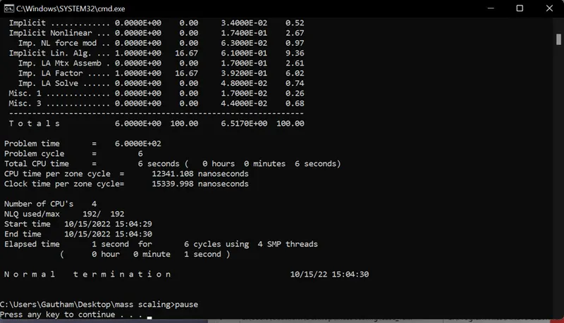
Now we will run this same file using an implicit solver. Additional control cards are used to run this simulation in an implicit solver.

CONTROL CARDS:

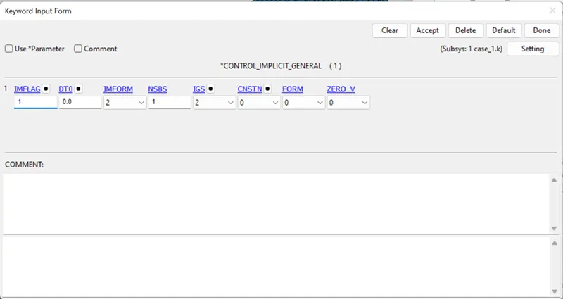
*CONTROL_IMPLICIT_GENERAL

Activate implicit analysis and define associated control parameters.

This keyword is required for all implicit analyses.

• IMFLAG - Implicit/Explicit analysis type flag: 1- implicit analysis.
• DT0 – Initial time step size for implicit analysis (Termination time/100): 
• IMFORM - Element formulation flag for seamless spring back: 2 retain original element formulation (default).

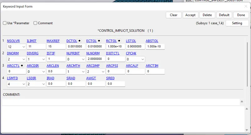
*CONTROL_IMPLICIT_SOLUTION

Use of these cards to specify whether a linear or nonlinear solution is desired.

• NSOLVER – Solution method for implicit analysis: 12 For Non-linear problem.
• ILIMIT-Iteration limit between automatic stiffness reformations: 11
• MAXREF- Stiffness reformation limit per time step: 15
• DCTOL- Displacement relative convergence tolerance:0.001
• DNORM- Displacement norm for convergence test: 2 (Increment as a function of total displacement)

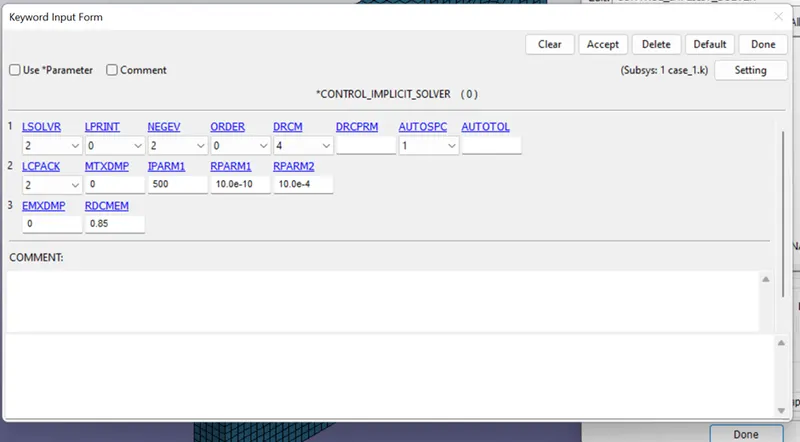
*CONTROL_IMPLICIT_SOLVER

The linear equation solver performs the CPU-intensive stiffness matrix inversion.

LSOLVR: Parallel multi-frontal sparse solver (default).

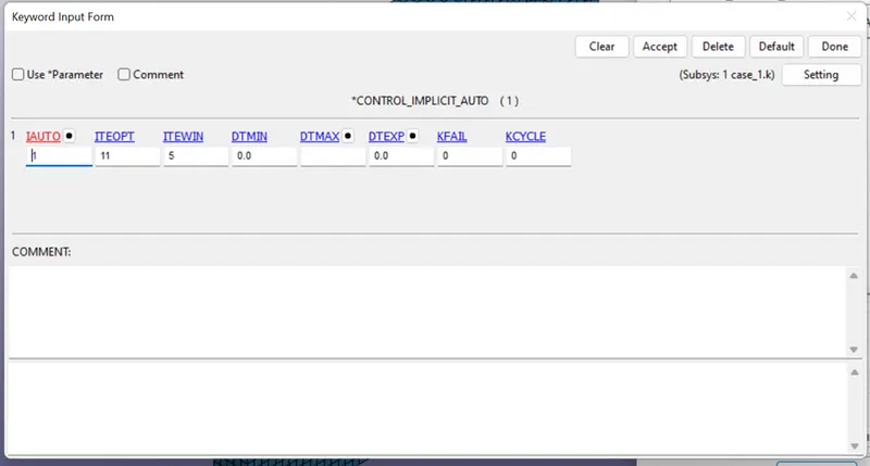
 *CONTROL_IMPLICIT_AUTO:

IAUTO: 1 - automatically adjust the time step size

ITEOPT: Optimum equilibrium iteration count per time step

ITEWIN: Allowable iteration window. If the iteration count is within ITEWIN iterations of ITEOPT, the step size will not be adjusted.

RESULT AND DISSCUSION:

TSSFAC	DT2MS	TIME ESTIMATION	MASS
0.9	-3.50E-05	23.44	0
0.9	-3.00E-05	11	0
0.9	-2.00E-05	14.26	0
0.9	-1.00E-05	9.37	0
0.9	-3.00E-04	2.34	7.24
0.9	-2.00E-04	2.11	2.72
0.9	-1.00E-04	5.23	6.42
0.9	-1.05E-04	7.03	10.74
0.9	-1.03E-04	7.21	8.06
0.9	-1.03E-04	5.33	8
0.8	-1.03E-04	5.31	8
0.7	-1.03E-04	11.02	8
0.6	-1.03E-04	11.21	8
0.5	-1.03E-04	10.36	8

The histogram plots were made for  Estimated Time VS DT2MS.

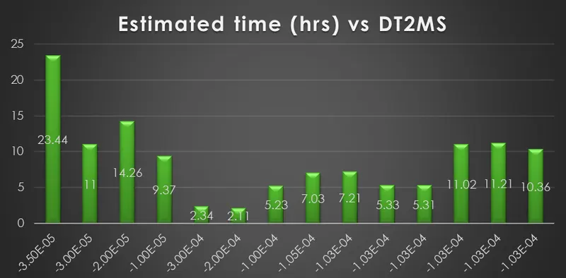
The  Estimated Time vs DT2MS  shows that when we add mass to the model using the DT2MS as the value of it increases the estimated simulation time decreases gradually.

MASS VS DT2MS :

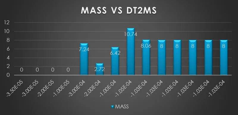
Here the DT2MS value is decreses  the mass is increases.

Estimated Tme vs TSSFAC:

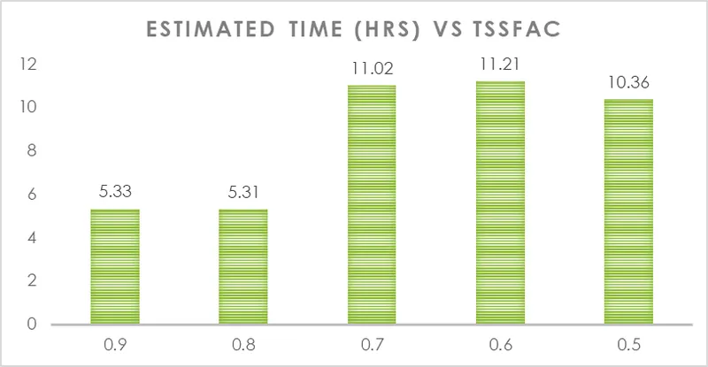
          It shows that when we don't vary the DT2MS value and change the TSSFAC values which don't add mass to the model as seen from the above cases the mass percentage remains the same because of which the estimated simulation time increases.

MASS VS TSSFAC: 

Comparison between explicit and implicit runtime:

   As we know, Explicit FEM is used to calculate the state of a given system at a different time from the current time. In contrast, an implicit analysis finds a solution by solving an equation that includes both the current and later states of the given system. In Implicit analysis, each time step has to converge, but we can set pretty long time steps and it is based on iterations. Explicit on the other hand doesn’t have to converge each time step, but for the solution to be accurate time steps must be small. Though the running time for implicit analysis is shorter than the explicit analysis method because the timestep is defined larger in implicit compare to explicit analysis and we have used constant timestep formulation. 

CONCLUSION:

• We have learned about the mass scaling Technique to reduce the computational time for the analysis.
• We can absorb the mass scaling percentage to 8% by varying the DT2MS values and then we have also found that TSSFAC  doesn't depend on the adding mass to the model.
• After, that we have run the analysis using implicit control cards which gives us the result that the implicit analysis is based on iterations and doesn't depend on mass scaling.
• Finally, we also compared explicit and implicit analysis, also we have plotted the histogram for  Estimated Time vs DT2MS and  Estimated Time vs TSSFAC.