Week - 2 - Explicit and Implicit Analysis

AIM; To slove the given equation with the Implicit and explicit methods with the proper tolerance value and write brief details about the Implicit and explicit method.

IMPLICIT METHOD	EXPLICIT METHOD
No effect of mass (inertia) or of damping.	Mass/inertia and damping are included.
Static analysis is done using an implicit solver.	Dynamic analysis can be done via the explicit solver.
solution of each step requires iterative solutions to establish equilibrium within a certain tolerance.	No iteration is required as the nodal accelerations are solved directly.
Time steps are generally larger than explicit time steps, Requires a numerical solver to invert the stiffness matrix once or even several times over the course of a load/time step, which is expensive for large models.	Time step must be less than the Courrant time step, Doses not require matrix inversion, Handles contact and material nonlinearities with relative easy.
In this Nertwon-Raphson enforce equilibrium are required.	Achieve Direct solution
Time consuming process.	computationally efficient for large models with relatively short dynamics time.
More accurate.	less accurate.

GIVEN EQUATION;

F(u) = u3+9u2+4u

From eqution(1) it follows the Stiffness of the bar,

K(u)=df/du

K(u)=3u^2+18u+4

EXPLICIT METHOD PROCESS;

Step1; u0=0`⇒`k(u0)=3(0)^2+18(0)+4(0)=4`

Delta F=1

`Deltau1= F/k(u0)=1/4=0.25`

`U1=u0+Deltau1=0+0.25=0.25`

Step2; `k(u1)=3(0.25)^2+18(0.25)+4(0.25)=8.68`

Delta F=1

`Deltau2= F/k(u0)=1/8.68=0.115`

`U2=u1+Deltau2=0.25+0.115=0.365`

Step3; `k(u2)=3(0.365)^2+9(0.365)+4(0.365)=8.4296`

Delta F=1

`Deltau3= F/k(u2)=1/8.4296=0.11862`

`U3=u2+Deltau3=0.365+0.11862=0.4836`

External & Internal Force Calculation:

Fext=DeltaF1+DeltaF2+DeltaF3

Fext=1+1+1=3

fint1= u1^3+9u1^2+4u1`

=(0.25)^3+9(0.25)^2+4(0.25)`

fint = 1.5781`

fint2= u2^3+9u2^2+4u2`

= (0.365)^3+9(0.365)^2+4(0.365)

fint = 2.7076`

fint3= u3^3+9u3^2+4u3`

=(0.48)^3+9(0.48)^2+4(0.48)

fint= 4

Step i	Delta Fi	Delta Ui	ui	(Fext)i	(fi)i	fint-Fext= R
1	1	0.25	0.25	1	1.5781	0.5781
2	1	0.115	0.365	2	2.7076	0.7076
3	1	0.118	0.483	3	4	1

Implicit Method :

The Implicit analysis is also the same as Explicit analysis except that at the end of each step Newton-Raphson iterations are used to enforce equilibrium before moving to the next step. Basically, an incremental force is applied to advance the solution forward at the beginning of the step.

However, internal forces and external forces will not be in equilibrium unless the stiffness is linear for the given timestep. Hence in order to achieve equilibrium, corrections must be made to the displacement.

This is accomplished by using Newton-Raphson iterations to minimize the residual,R(u)=fInt−Fext.

By expanding the Newton-Raphson iterations to minimize the residual to a simpler form.

δu^j+1=-[K(uj)]-1⋅R^j

Step1;

u0=0.0, K(u0) =3(0)2+18(0)+4 =4

Delta F=1

`Deltau1= F/k(u0)=1/4=0.25`

`U1=u0+Deltau1=0+0.25=0.25`

Check the residual, fint=u^3+9u^2+4u

Where Keep U1=0.25 in the above equation.

fint=(0.25)^3+9(0.25)^2+4(0.25)=1.578

Fext=1

Resudial(R0)=Fint- Fext=1.578-1=0.578

Where||R0||=0.578 is greater than 0.001.So, we need to do Newton raphson method iteration.

Calculate the correction to u1 = u1^(0)

δu(1) = −[k(u1^(0)]^-1R(0)

substitute U1=0.25

k(u1^(0))=3(0.25)^2+18(0.25)+4=8.687

δu1=−(8.687)^-1x0.578=-0.06653

⇒ The updated value of u1^(1)= u1^(0) + δu(1)

u1 =0.25-0.06653=0.1834

Check the residual again, Fext = 1, fint =(0.183)^3+9(0.183)^2+4(0.183)=1.043

Resudial(R1)=fint-Fext=1.043-1=0.043.

||R(1)||> 0.01 ⇒ another Newton-Raphson iteration is necessary.

Calculate the new total correction to u1 = u1^(0)

δu(2) = δu(1) − [k(u1^(1)]^−1R(1)

[k(u1^(1)]^−1= k(u01)=3(0.183)^2+18(0.183)+4=7.394

δu(2)=-0.06653-(7.394)^-1x(0.043)

δu(2) =-0.0723

The updated value of u1^(2)= u1^(0)+ δu(2)

u1^(2)=0.25-0.0723=0.1777

Check the residual, Fext = 1, fint=(0.1777)^3+9(0.1777)^2+4(0.1777)=1.00060

R(2) = fint − Fext = 0.0006

||R(1)||< 0.001 ⇒no further iterations are necessary.

Therefore, the final value is u1 = u1^(2)= 0.1777

Step2;

K(u1)=3u^2+18u+4,

K(u1)=3(0.1777)^2+18(0.1777)+4

K(u1)=7.2933

DeltaF2=1

Deltau2= (DeltaF2)/(K(u1))=0.1371

`u2=u1+Deltau2

=0.1777+0.1371

u2=0.3148

Check the residual

Fext=2,`

fint=u^3+9u^2+4u

= (0.3148)^3+9(0.3148)^2+4(0.3148)=2.1822

fin=2.1822

R0=fint−Fext=2.1822-2=0.1822

||R(1)||> 0.001- Newton-Raphson iterations are necessary.

Calculate the correction to u2=u2^(0)

δu1=−[k(u2^(0)]^-1R(0)

K(u2)=3u2+18u+4

=3(0.3148)^2+18(0.3148)+4=9.9636

δu1=−[K(u2^(0)]^−1⋅R0

δu1=-(9.9636)^-1*(0.1822)

δu1=−0.0183

The updated value of u2^(1)=u2+δu1

u2^(1)=0.3148−0.0183=0.2965

Check the residual again,Fext=2;

fint=(u2)3+9(u2)2+4(u2)

=2.0032

R1=fint−Fext

R1=2.0032−2

R1=0.0032

||R(2)||> 0.001

STEP3

K(u2)=3u^2+18u+4,

K(u2)=3(0.2965)^2+18(0.2965)+4

K(u2)=9.6007

DeltaF3=1

Deltau3= (DeltaF3)/(K(u2))=0.1041

`u3=u2+Deltau3

=0.2965+0.1041

u3=0.4006

Check the residual

Fext=3,`

fint=u^3+9u^2+4u

= (0.4006)^3+9(0.4006)^2+4(0.4006)=3.1110

R0=fint−Fext=3.1110-3=0.1110

||R(1)||> 0.001- Newton-Raphson iterations are necessary.

Calculate the correction to u3=u3^(0)

δu1=−[k(u3^(0)]^-1R(0)

K(u3)=3u2+18u+4

=3(0.4006)^2+18(0.4006)+4=11.6922

δu1=−[K(u2^(0)]^−1⋅R0

δu1=-(11.6922)^-1*(0.1110)

δu1=−0.0095

The updated value of u3^(1)=u3+δu1

u3^(1)=0.4006−0.0094=0.3911

Check the residual again,Fext=3;

fint=(u3)3+9(u3)2+4(u3)

=3.00085

R2=fint−Fext

R2=3.00085−3

R2=0.00085

||R(2)||<0.001⇒ no further iterations are necessary.

Therefore, the final value is u3^(1)= 0.3911

Step i	Delta Fi	ui	(Fext)i	(fi)i	fint-Fext= R
1	1	0.1777	1	1.00060	0.0006
2	1	0.2965	2	2.0032	0.0032
3	1	0.3911	3	3.00085	0.00085

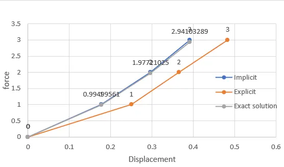
The below chart indicates the Force vs Displacement curves of the Implicit and Explicit methods.

CONCLUSION;

• From the above plot we can conclude the results such as.
• It says that is very evident from the plot that the explicit analysis drifts from the exact solution.
• The drift from the exact solution illustrates the lack of equilibrium between the internal and external forces.
• To correct for this problem an implicit analysis is required. The results for the implicit analysis are shown in Figure .
• The Newton-Raphson iterations correct the incremental steps so that they land on the exact solution according to the specified tolerance.