Week 3 - Solving second order ODEs

AIM;

To create a simple pendulum in a Matlab for a second-order differential equation.

EQUATIONS USED;

`(d^2 theta)/dt^2+b/m (d theta )/ dt +g/lsintheta =0`

Here

gravity(g)=9.81m/s^2

length of the pendulum(l)=1m

mass of the bob(m)=1kg

beam coefficient(b)=0.05

displacement=0

angular velocity=3rad/sec

Time span(t_span)=0-20sec

OBJECTIVES;

To write an program that sloves an ODEs which represents the motion of a simple pendulum.

THEORY;

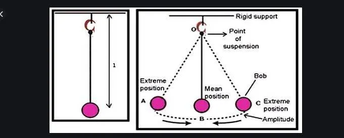
• A simple pendulum is a weight suspended from a beam on which that can swing freely which was shown in the above figure.
• The simple pendulum consists of a mass of the bob, spring length, beam support, and some opposing forces to the gravity.
• when a pendulum is displaced sideways from its rest position and it tends to move from the mean position to the extreme position and it is subject to some restoring force due to the gravity that will accelerate its to the mean position.
• When it is released the mass of the bob will cause oscillations and make a certain displacement and angular velocity of the pendulum.
• The time is taken for one complete cycle that from the left and right swing is called a period and the period depends on the length of the pendulum and also the slight degree to the amplitude.
• The period of a simple pendulum is `T=2pisqrt(l/g)`.

CODE;

It is a call function that was used in the main code.

function[dtheta_dt]=ode_func(t, theta, b, g, l, m)
theta1 = theta(1);
theta2 = theta(2);
dtheta1_dt=theta2;
dtheta2_dt=-(b/m)*theta2-(g/l)*sin(theta1);
dtheta_dt=[dtheta1_dt;dtheta2_dt];

end

CODE;

Main Code

clear all
close all
clc
b=0.05;
g=9.81;
l=1;
m=1;

%Initial conditions
theta=[0;3];

%time points
t_span=linspace(0,20,100);

%slove ode
[t,results]=ode45(@(t,theta) ode_func(t, theta, b, g, l, m),t_span,theta);

% plot(t,results(:,1));
% hold on
% plot(t,results(:,2));
% 
% xlabel('time');
% ylabel('plot');

ct=1;
for i=1:length(t_span);

x0=0;
y0=0;
x1=l*sin(results(i,1));
y1=-l*cos(results(i,1)) ;
figure(ct);
%plotting
hold on
plot([x0 x1],[y0 y1]);
 plot(x1, y1,'marker','o','markerfacecolor','g');
axis([-1 1  -1.2 1]);
pause(0.3)
M(ct)=getframe(gcf);
ct=ct+1;
end
movie(M)
videofile=VideoWriter('pendulum.avi','uncompressed AVI');
open(videofile)
writeVideo(videofile,M)
close(videofile)


    
    
    

PLOT RESULT;

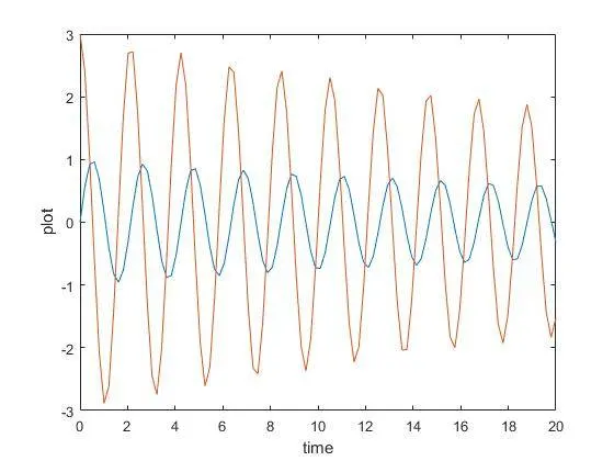
ANIMATION VIEW OF AN SIMPLE PENDULUM;

https://youtu.be/mJZyKxEDJKw

PROCEDURE;

1. Firstly the given input data is taken into the code part and set the initial conditions of the displacement, angular velocity as the theta, and time span can be set by using a linspace command.
2. After this, we can make an ode45 function which has taken from an ode_func function which called for the main function code in order to solve the ode45 program.
3. By using the plot command we plot the graph to the displacement and angular velocity of the simple pendulum by using a column vector.
4. Next we use a for loop command in order to set the start and endpoints of the pendulum and help in making as an animation part.
5. First, we denote the origin axis (x0 y0) and end axis of the pendulum (x1 y1) and finally make a bob by using a marker command and denote as a particular color to it.
6. Axis should be given and create a video file to the pendulum.

CONCLUSION;

We create a simple pendulum by considering the odes and made an animation view of the simple pendulum.