Week 12 - Symmetry vs Wedge vs HP equation
Theory:
The comparison between the wedge boundary condition and symmetry boundary condition are very timming and make more confusion. The only part which need to be understant is utilization of both boundary condition for specifc cases.
The wedge boundary condition for openFoam is suitable for the angle less than 5 degree and only supports for the 2D axi-symmetric cases, whereas the symmetric boundary condition are can be use for multiple cases including 2D and 3D geometry.
In the challenge we have to compare the wedge boundary condition with symmetric boundary conditions with different angle. The code or file for the simulation will be the same only the for symmetric boundary conditions instead of wedge we will use symmetry for the front and back faces.
The objective of the challege are given as:
1) To create the parsing file for blockMeshDict file using symmetry boundary condition.
2) To simulate the Hagen-Poisuelle equation for different angles usign symmetry boundary conditions.
3) To compare the results of wedge angles determined in challenge 10 with the symmetry boundary conditions results.
4) To comment on the observation of the results.
Objective 1
The input for the equation will be the same for challenge 11 which are given as:
1) Density of Water = 1000 kg/m3.
2) Dynamic Viscosity = 8.9e-4 Pa.s
3) Reynolds Number = 2100
4) Diameter of pipe = 0.01 m
5) Inlet velocity = 0.1869 m/s
Outputs calculation from Hagen-Poisuelle equations.
1) Average velocity = `V_(avg) = (Re.U)/(Rho*D) = 0.1869 ms^-1`
2) Maximum velocity = `V_(max) = 2. V_(avg) = 0.3738 ms^-1`
3) Pressure drop = `Delta P = (32*mu*L*V_(avg))/(D^2) = 63.8749 Pa`
4) Kinematic Pressure = `Delta P^k = (DeltaP)/(rho) = 0.063874 m^2 s^-2`
5) Length of Pipe = 1.2 Meters.
The MATLAB code for Parsing file for Symmetry BC is given as:
clear all
close all
clc

%Considering Reynold's Number for Simulation
re = 2100;
% Consideration Diameter of Pipe from the equation
D = 0.01;
%Radius of pipe
r = D/2;
%Total length of Pipe is given as
L_t = 1.2;
%Considering angle of wedge (should be < 5)
theta = 10;
% Considering dynamic viscosity
mu = 0.89e-3;
% Density of fluid (kg/m3)
Rho = 1000;

% Deriving variable from Hagen poiseuille equation
v_avg = (re*mu)/(Rho*D);        % Average Velocity
v_max = 2*(v_avg);              % Maximum Velocity
Del_p = (8*mu*L_t*v_avg)/(r^2); % Pressure difference
k_p = Del_p/Rho;                % Kinematic Pressure

% Calculating Shear stress
R = linspace(0,r,1000);

for i = 1:length(R)
    tau(i) = 2*mu*v_max*(abs(R(i)))/r^2;
end

plot(R,tau)
xlabel('Radius')
ylabel('Shear Stress')
grid on
legend ('Shear stress in Pipe')

header1='/*--------------------------------*- C++ -*----------------------------------*\';
header2='  =========                 |                                                  ';
header3='  \\      /  F ield         | OpenFOAM: The Open Source CFD Toolbox            ';
header4='   \\    /   O peration     | Website:  https://openfoam.org                   ';
header5='    \\  /    A nd           | Version:  8                                      ';
header6='     \\/     M anipulation  |                                                  ';
header7='\*---------------------------------------------------------------------------*/';

f1 = fopen('blockMeshDict','w');
fprintf(f1, '%s\n', header1);
fprintf(f1, '%s\n', header2);
fprintf(f1, '%s\n', header3);
fprintf(f1, '%s\n', header4);
fprintf(f1, '%s\n', header5);
fprintf(f1, '%s\n', header6);
fprintf(f1, '%s\n', header7);

fprintf(f1, 'FoamFile\n{\n');
fprintf(f1, '%12s \t 2.0;\n', 'version');
fprintf(f1, '%12s \t ascii;\n','format');
fprintf(f1, '%12s \t dictionary;\n','class');
fprintf(f1, '%12s \t blockMeshDict;\n','object');
fprintf(f1, '}\n');
header8='// * * * * * * * * * * * * * * * * * * * * * * * * * * * * * * * * * * * * * //';
fprintf(f1, '%s\n\n',header8);

fprintf(f1, 'convertToMeters 1;\n\n');

fprintf(f1, 'vertices\n');
fprintf(f1, '(\n');
fprintf(f1, '\t (%d  %d %d)\n',0,0,0);
fprintf(f1, '\t (%d  %d %d)\n',r*sind(theta/2),r*cosd(theta/2),0);
fprintf(f1, '\t (%d  %d %d)\n',-r*sind(theta/2),r*cosd(theta/2),0);
fprintf(f1, '\t (%d  %d %d)\n',0,0,L_t);
fprintf(f1, '\t (%d  %d %d)\n',r*sind(theta/2),r*cosd(theta/2),L_t);
fprintf(f1, '\t (%d  %d %d)\n',-r*sind(theta/2),r*cosd(theta/2),L_t);
fprintf(f1, ');\n\n');


fprintf(f1, 'blocks\n');
fprintf(f1, '(\n');
fprintf(f1, '\t hex (0 0 1 2 3 3 4 5) (%d %d %d)',1,50,300);
fprintf(f1, ' SimpleGrading (1 0.5 1)\n\n');
fprintf(f1, ');\n\n');

fprintf(f1, 'edges\n');
fprintf(f1, '(\n');
fprintf(f1, '\t arc %d %d (%d %d %d)\n',1,2,0,r,0);
fprintf(f1, '\t arc %d %d (%d %d %d)\n',4,5,0,r,L_t);
fprintf(f1, ');\n\n');

fprintf(f1, 'boundary\n');
fprintf(f1, '(\n');
fprintf(f1, '\t inlet\n');
fprintf(f1, '\t {\n');
fprintf(f1, '\t\t type patch;\n');
fprintf(f1, '\t\t faces\n');
fprintf(f1, '\t\t (\n');
fprintf(f1, '\t\t\t (0 0 2 1)\n');
fprintf(f1, '\t\t );\n');
fprintf(f1, '\t }\n');


fprintf(f1, '\t outlet\n');
fprintf(f1, '\t {\n');
fprintf(f1, '\t\t type patch;\n');
fprintf(f1, '\t\t faces\n');
fprintf(f1, '\t\t (\n');
fprintf(f1, '\t\t\t (3 4 5 3)\n');
fprintf(f1, '\t\t );\n');
fprintf(f1, '\t }\n');

fprintf(f1, '\t top\n');
fprintf(f1, '\t {\n');
fprintf(f1, '\t\t type wall;\n');
fprintf(f1, '\t\t faces\n');
fprintf(f1, '\t\t (\n');
fprintf(f1, '\t\t\t (4 1 2 5)\n');
fprintf(f1, '\t\t );\n');
fprintf(f1, '\t }\n');


fprintf(f1, '\t front\n');
fprintf(f1, '\t {\n');
fprintf(f1, '\t\t type symmetry;\n');
fprintf(f1, '\t\t faces\n');
fprintf(f1, '\t\t (\n');
fprintf(f1, '\t\t\t (0 1 4 3)\n');
fprintf(f1, '\t\t );\n');
fprintf(f1, '\t }\n');


fprintf(f1, '\t back\n');
fprintf(f1, '\t {\n');
fprintf(f1, '\t\t type symmetry;\n');
fprintf(f1, '\t\t faces\n');
fprintf(f1, '\t\t (\n');
fprintf(f1, '\t\t\t (3 5 2 0)\n');
fprintf(f1, '\t\t );\n');
fprintf(f1, '\t }\n');

fprintf(f1, '\t axis\n');
fprintf(f1, '\t {\n');
fprintf(f1, '\t\t type empty;\n');
fprintf(f1, '\t\t faces\n');
fprintf(f1, '\t\t (\n');
fprintf(f1, '\t\t\t (0 3 3 0)\n');
fprintf(f1, '\t\t );\n');
fprintf(f1, '\t }\n');
fprintf(f1, '); \n\n');

fprintf(f1, 'mergePatchPairs\n');
fprintf(f1, '(\n');
fprintf(f1, ');\n');

header9='// ************************************************************************* //';
fprintf(f1, '%s\n',header9);

fclose(f1);
After running the MATLAB code we will get the blockMeshDict file as:
/*--------------------------------*- C++ -*----------------------------------*\
  =========                 |
  \\      /  F ield         | OpenFOAM: The Open Source CFD Toolbox
   \\    /   O peration     | Website:  https://openfoam.org
    \\  /    A nd           | Version:  8
     \\/     M anipulation  |
\*---------------------------------------------------------------------------*/
FoamFile
{
     version 	 2.0;
      format 	 ascii;
       class 	 dictionary;
      object 	 blockMeshDict;
}
// * * * * * * * * * * * * * * * * * * * * * * * * * * * * * * * * * * * * * //

convertToMeters 1;

vertices
(
	 (0  0 0)
	 (4.357787e-04  4.980973e-03 0)
	 (-4.357787e-04  4.980973e-03 0)
	 (0  0 1.200000e+00)
	 (4.357787e-04  4.980973e-03 1.200000e+00)
	 (-4.357787e-04  4.980973e-03 1.200000e+00)
);

blocks
(
	 hex (0 0 1 2 3 3 4 5) (1 50 300) SimpleGrading (1 0.5 1)

);

edges
(
	 arc 1 2 (0 5.000000e-03 0)
	 arc 4 5 (0 5.000000e-03 1.200000e+00)
);

boundary
(
	 inlet
	 {
		 type patch;
		 faces
		 (
			 (0 0 2 1)
		 );
	 }
	 outlet
	 {
		 type patch;
		 faces
		 (
			 (3 4 5 3)
		 );
	 }
	 top
	 {
		 type wall;
		 faces
		 (
			 (4 1 2 5)
		 );
	 }
	 front
	 {
		 type symmetry;
		 faces
		 (
			 (0 1 4 3)
		 );
	 }
	 back
	 {
		 type symmetry;
		 faces
		 (
			 (3 5 2 0)
		 );
	 }
	 axis
	 {
		 type empty;
		 faces
		 (
			 (0 3 3 0)
		 );
	 }
);

mergePatchPairs
(
);
// ************************************************************************* //
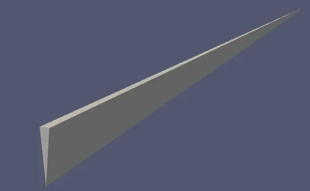
Geomtry for Theta = 10.
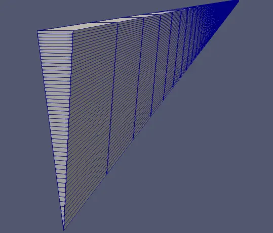
Meshing for Theta 10
Objective 2
Similarly Initial Condition are change for simulation which are given by:
For pressure condition,
/*--------------------------------*- C++ -*----------------------------------*\
  =========                 |
  \\      /  F ield         | OpenFOAM: The Open Source CFD Toolbox
   \\    /   O peration     | Website:  https://openfoam.org
    \\  /    A nd           | Version:  8
     \\/     M anipulation  |
\*---------------------------------------------------------------------------*/
FoamFile
{
    version     2.0;
    format      ascii;
    class       volScalarField;
    object      p;
}
// * * * * * * * * * * * * * * * * * * * * * * * * * * * * * * * * * * * * * //

dimensions      [0 2 -2 0 0 0 0];

internalField   uniform 0;

boundaryField
{
    inlet
    {
        type            zeroGradient;
    }

    outlet
    {
        type            fixedValue;
        value		 uniform 0.063874;
    }

    top
    {
    	type		 zeroGradient;
    }

    front
    {
        type            symmetry;
    }

    back
    {
    	type            symmetry;
    }

    axis
    {
    	type		 empty;
    }
}

// ************************************************************************* //
For Velocity Boundary Condition.
/*--------------------------------*- C++ -*----------------------------------*\
  =========                 |
  \\      /  F ield         | OpenFOAM: The Open Source CFD Toolbox
   \\    /   O peration     | Website:  https://openfoam.org
    \\  /    A nd           | Version:  8
     \\/     M anipulation  |
\*---------------------------------------------------------------------------*/
FoamFile
{
    version     2.0;
    format      ascii;
    class       volVectorField;
    object      U;
}
// * * * * * * * * * * * * * * * * * * * * * * * * * * * * * * * * * * * * * //

dimensions      [0 1 -1 0 0 0 0];

internalField   uniform (0 0 0);

boundaryField
{
    inlet
    {
        type            fixedValue;
        value		 uniform (0 0 0.1869);
    }

    outlet
    {
        type            zeroGradient;
    }

    top
    {
    	type		 noSlip;
    }

    front
    {
        type            symmetry;
    }

    back
    {
    	type            symmetry;
    }

    axis
    {
    	type		 empty;
    }
}

// ************************************************************************* //
The ControlDict File
/*--------------------------------*- C++ -*----------------------------------*\
  =========                 |
  \\      /  F ield         | OpenFOAM: The Open Source CFD Toolbox
   \\    /   O peration     | Website:  https://openfoam.org
    \\  /    A nd           | Version:  8
     \\/     M anipulation  |
\*---------------------------------------------------------------------------*/
FoamFile
{
    version     2.0;
    format      ascii;
    class       dictionary;
    location    "system";
    object      controlDict;
}
// * * * * * * * * * * * * * * * * * * * * * * * * * * * * * * * * * * * * * //

application     icoFoam;

startFrom       startTime;

startTime       0;

stopAt          endTime;

endTime         10;

deltaT          0.005;

writeControl    timeStep;

writeInterval   20;

purgeWrite      0;

writeFormat     ascii;

writePrecision  6;

writeCompression off;

timeFormat      general;

timePrecision   6;

runTimeModifiable true;


// ************************************************************************* //
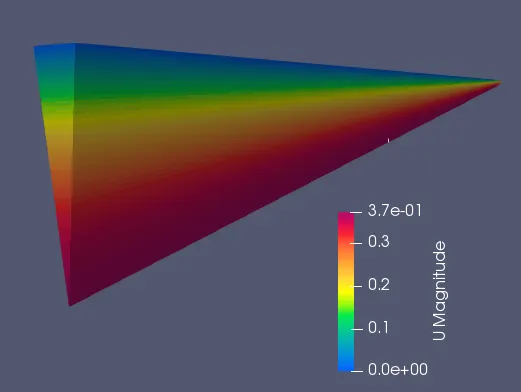
Results for Theta 10
A) Velocity Contour
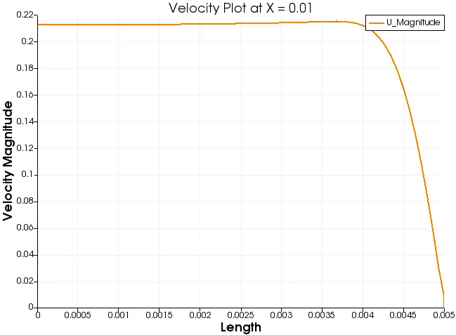
B) Plot of Velocity at X = 0.01
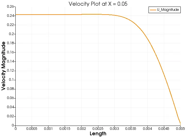
C) Plot of Velocity at X = 0.05
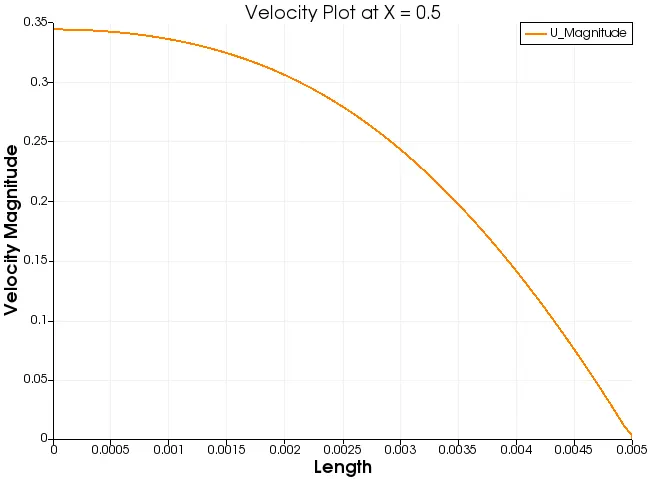
D) Plot of Velocity at X = 0.5
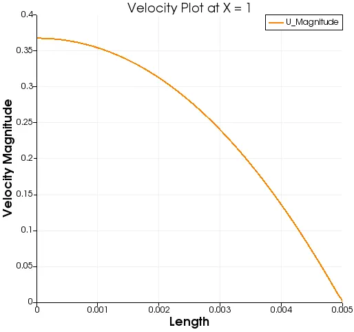
E) Plot of Velocity at X = 1
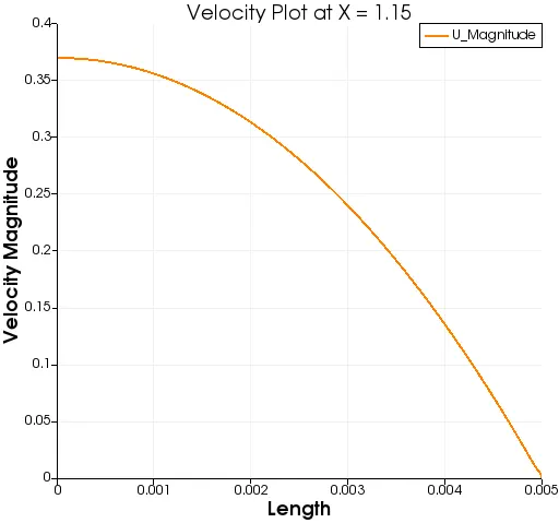
F) Plot of Velocity at X = 1.15
Objective 3
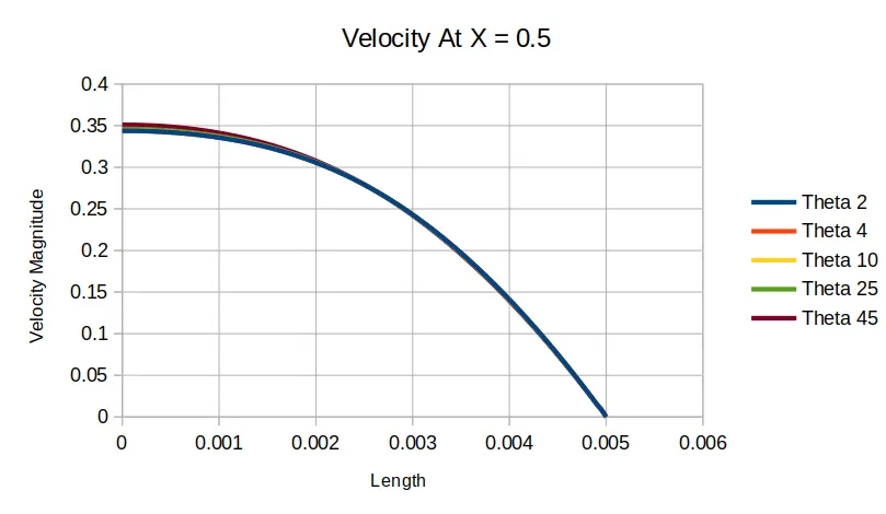
Results for Theta 2, 4, 10, 25 and 45 at X = 0.5
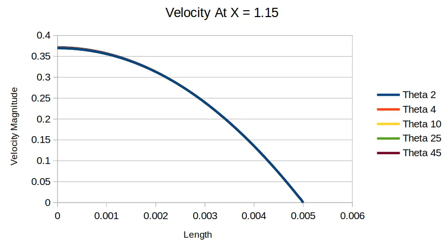
Results for Theta 2, 4, 10, 25 and 45 at X = 1.15
Result Table
| Value of Theta | Numerical Velocity Maximum (m/s) | Analytical Velocity Maximum (m/s) | Error | Time For Simulation |
| 2 | 0.37022 | 0.3738 | 0.957 | 359 |
| 4 | 0.370231 | 0.3738 | 0.954 | 357 |
| 10 | 0.370309 | 0.3738 | 0.933 | 391 |
| 25 | 0.370765 | 0.3738 | 0.811 | 398 |
| 45 | 0.371764 | 0.3738 | 0.544 | 391 |
Objective 4:
1) We have compared the wegde boundary condition and symmetry boundary condition for problem, as we can see from the graph the symmetry boundary condition gives more accurate value for same number of theta.
2) The parabolic curve will be reaching earlier and in case of symmetry boundary conditions.
3) The error value is lesser in case of symmetry boundary condition.
4) The time elapsed for the simulation is more in case of symmetry boundary condition for same of number of mesh parameters.