Week 3 - Solving second order ODEs

Simple Pendulum

Aim:

Solving a second order ordinary differential equation of simple pendulum and showing the effect of damping by an animation.

Objective:

• To convert second order ordinary differential equation to 1^st order ordinary differential equation.
• To create the function using Python in-built function for solving ordinary differential equation.
• To plot the displacement and velocity damping through the time stipulated time of simulation.
• To make the animation of simple pendulum.

Description & Governing equation.

The differential equation is mostly used to define the complex physics phenomenon in the mathematical way. Differential equation is divided in two different classify as ordinary differential equation and partial differential equation. Solving a 1^st order differential is quite easy and require only one constant to define the equation, also it can be also programmed easily. The main effort is taken while solving 2^nd order differential equation. Most of the fluid equation and some structural phenomenon are defined in the 2^nd order differential equation which need to solve eventually to simulated the flow or study the structural behavior.

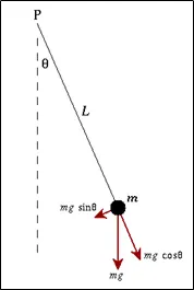
A simple pendulum consists of mass which is attached by the string of length L from a pivot point P. when displaced by initial force the mass gets moved back and forth performing periodic motion. By applying the Newton’s second law motion we can obtain the equation of motion for simple pendulum which is given as:

`(d^2 θ)/dt+b/m (dθ1)/dt+g/L sinθ= 0`

Consider `θ=θ1`

Then new equation of motion can be written as:

`(d^2 θ1)/(dt^2 )+b/m (dθ1)/dt+g/L sin⁡θ1 =0`

Consider,

`(dθ1)/dt=θ2`

Therefore, new equation can be written as:

`(dθ2)/dt+b/m θ2+g/L sin⁡θ1=0`

Which leads to:

`(dθ2)/dt= -b/m θ2-g/L sin⁡θ1`

The resultant first order equation will be:

`θ_1^'=θ2` and `θ_2^'= -b/m θ2-g/L sin⁡θ1`

Code explanation: -

• The code starts with the inputs which are provided in the problems. Then we make time domain for which the whole code is going to run. It was done by ‘linspace’ command from 0 to 20 seconds with 100 value in between them.
• After that we provide the initial condition for the angular displacement and velocity which is column vector form, because we need to calculate the both value from the equation of motion for plotting purpose.
• The code comprises of function which solves the second order differential equation which is taken inside the main code. The main code has another function which calculates the array of data for time and displacement.
• After calculation plotting is done in which subplot command is used, in the first plot first column is plotted and in second subplot second column is plotted with respect to time.
• Then we have created a for loop for which we are creating the frame motion for the simple pendulum and saved in the movie.

"""
Week 3 Challenge - Solving Second Order ODE of Simple Pendulum
Written By: Shubham K Chaudhari
Date : - 25the August 2021
"""
import math
import matplotlib.pyplot as plt
import numpy as np
from scipy.integrate import odeint

# Defining function for input of ODE


def ode_func(theta,t,b,g,l,m):
    theta1 = theta[0]
    theta2 = theta[1]
    dtheta1_dt = theta2                                 # First Order
    dtheta2_dt = -(b/m)*theta2-(g/l)*math.sin(theta1)   # Second Order simplification
    dtheta_dt = [dtheta1_dt,dtheta2_dt]
    return dtheta_dt

# Inputs for Simulation of Simple Pendulum
b = 0.05        # Damping Coefficients
g = 9.81        # Acceleration Due to Gravity
l = 1           # Length of string
m = 1           # Mass of bob

# Initial time parameters
theta_0 = [0,3]
t_span = np.linspace(0,20,100)

# Solving ODE
theta = odeint(ode_func,theta_0,t_span,args=(b,g,l,m))

# Plotting of Results
plt.plot(t_span,theta[:,0],'b-',label= r'$\frac{d\theta1}{dt}=\theta2$')
plt.plot(t_span,theta[:,1],'r--',label = r'$\frac{d\theta2}{dt}=-\frac{b}{m}\theta2-\frac{g}{l}sin\theta1$')
plt.xlabel('Time in Second')
plt.ylabel('Plot')
plt.title('Damped Vibration of Simple Pendulum')
plt.legend(loc='best')
plt.grid()
plt.show()

# Animation of Pendulum
loop_counter = 1
tmp = theta[:,0]
for i in tmp:
    x_start = 0
    y_start = 0
    x_end = l*math.sin(i)
    y_end = -l*math.cos(i)
    # Plotting For Animation
    plt.figure()
    plt.plot([x_start,x_end],[y_start,y_end],linewidth = 3)
    plt.plot(x_end,y_end,'o',markersize=20,color='r')
    plt.plot([-0.5,0.5],[0,0],linewidth=8,color='k')
    plt.plot([0,0],[0,-1.5],'--',color = 'y')
    plt.xlim([-1.25,1.25])
    plt.ylim([-2,1])
    plt.title('Animation of Simple Pendulum')
    filename = '%d.png' %loop_counter
    plt.savefig(filename)
    loop_counter = loop_counter + 1

Results

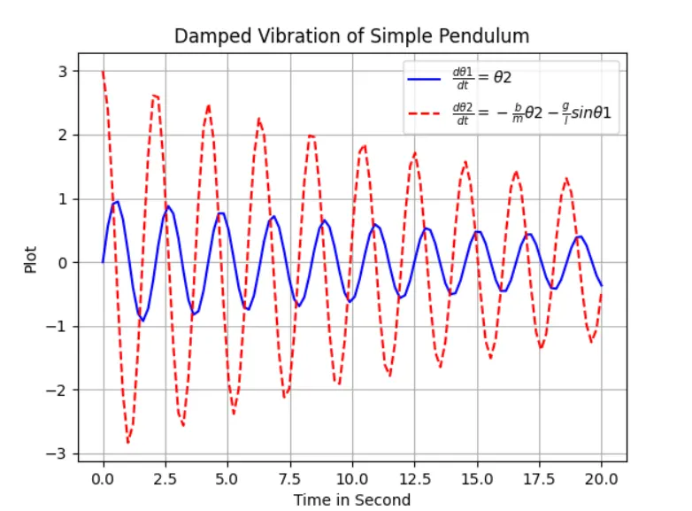
1) Plot for Damping of Velocity and Displacement

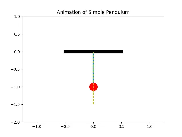
2) Animation of Simple Pendulum

3) Animation Video Link

https://youtu.be/QvVTaC-8I8s

Inference of Plot:

As we can see from the plots the displacement is getting reduce as we move further in to time because of damping factor. From the plot we can clearly observe displacement is starting from 0 as initial condition. In the angular velocity vs time plot it has started from 3 rad/sec and then further get decrease.

Conclusion: -

From the graph and from the animation we can see that we have clearly simulate the equation of motion for simple pendulum. No errors were encounterd during the code. The warning message has been shown while generating more than 20 image files.