Week 7 - Auto ignition using Cantera
Week 7: - Auto-Ignition Temperature Using Cantera Reactor Network
Aim: - Determination of Auto-ignition temperature for methane-air reaction for constant pressure & temperature conditions.
Objectives: -
- To study the Auto-ignition fundamentals and ignition delay.
- To determine the Auto-ignition temperature at constant temperature with varying pressure.
- To determine the Auto-ignition temperature at constant pressure with varying temperature.
- To determine the molar mass of H2O, OH and O2 at 500K and 1000K.
Introduction: -
Fuel and air need the specific temperature to combust on their own. It is well knowing that for spark ignition engine it required to have external heat source to create combustion whereas in diesel engine the spark plug is not required. The diesel engine mostly need to have fuel to burn automatically when certain temperature & pressure reached. In case of diesel engine, the fuel is introduced as highly pressurized via injector whereas in high compression combustion engine it is auto-ignition which play important role.
The auto-ignition is the lowest temperature at which the fuel burn spontaneously without addition of any heat in process. Auto-ignition is achieved at certain pressure and temperature also chemical ratio of fuel and air. If the temperature is right and proportion is not correct the auto-ignition won’t be happening. Similarly, if the right proportion is achieved but temperature for combustion is not reached then auto-ignition is not going to happen. Depending upon auto-ignition the ignition delay can be calculated. Ignition delay is the time required for ignition to take place. This delay time is an important function for the design of engine and mostly determined experimentally using shock-tube and Rapid Compression Machine. Ignition delay temperature is a parameter which typically varies with temperature, pressure, fuel to air ratio and type of fuel used.
Coding Approach Part 1 & 2: -
In first and second part of the coding, auto-ignition temperature is being evaluated based on the constant temperature with varying pressure and constant pressure with varying temperature respectively. The auto-ignition temperature is evaluated using Cantera and program is made in python. The modules of ‘matplotlib.pyplot’ and ‘numpy’ is being introduced in the code to make plotting and arithmetic operation respectively. For the first part the temperature is kept constant and pressure is varied from 1 to 5 atmospheric pressure. To have the auto-ignition temperature at every pressure the code has five variables which will stored the value of temperature. The first line of code is calling the object from cantera which is ‘gri30’. This object is an optimized mechanism designed to model the natural gas combustion. Then properties of gas are defined which is methane combustion with CH4 as 1 mole. Then a variable ‘r’ is created which have Ideal gas reactor class which is used for a constant volume chamber for zero dimensional reactor of ideal mixtures. Then ‘states’ variable is called in for storing the auto-ignition temperature in milliseconds. Then another loop is created for creation of time interval for first loop. The conditions are applied to get the value of auto-ignition temperature for particular atmospheric pressure. The similar coding approach is used for the second part the only difference is made in temperature and pressure variables. In second part the pressure is kept constant at 5 bar and the temperature is varying from 950 K to 1450 K. The simultaneous changes have been made in the code which will provide the auto-ignition temperature at different fuel temperature. The code for part 1 and 2 is shown below:
Part 1: -
"""
Determining Auto Ignition Temperature Using Cantera
Part 1: - Calculating Auto Ignition Time of Methane at Constant Temperature of 1250K
and pressure varying from 1 to 5 bar
Simulation time is 10 seconds
Properties of Fuel: CH4:1 moles, O2: 2 moles and N2: 7.52 moles
Code Written by: Shubham Chaudhari
Skill Lync Challenge Week 7
"""
import sys
import cantera as ct
import matplotlib.pyplot as plt
import numpy as np

# Creation of Gas object
gas = ct.Solution('gri30.xml')
T = 1250                                # specification of temperature
P = np.linspace(101325, 5*101325, 6)    # Specification of Pressure
time = np.zeros(5)                      # Defining list of time
auto_igni_time = []
# Different Pressure variable for saving auto ignition time
states_p1 = []
states_p2 = []
states_p3 = []
states_p4 = []
states_p5 = []

for i in range(5):
    gas.TPX = T, P[i], {'CH4':1,'O2':2,'N2':7.52}
    r = ct.IdealGasReactor(gas)
    sim = ct.ReactorNet([r])
    states = ct.SolutionArray(gas,extra=['time_in_ms','t'])

    for j in range(100):
        time[i] += 1e-3
        sim.advance(time[i])
        states.append(r.thermo.state, time_in_ms = time[i]*1e3, t = time[i])

# Use of Condition for storing different value of pressure
    if i == 0:
        states_p1 = states.T

    if i == 1:
        states_p2 = states.T

    if i == 2:
        states_p3 = states.T

    if i == 3:
        states_p4 = states.T

    if i == 4:
        states_p5 = states.T

plt.figure(1)
plt.plot(states.t, states_p1)
plt.plot(states.t, states_p2)
plt.plot(states.t, states_p3)
plt.plot(states.t, states_p4)
plt.plot(states.t, states_p5)
plt.title('Constant Temperature Effect on Pressure varying from 1 to 5 bar')
plt.xlabel('Ignition Delay in Seconds')
plt.ylabel('Auto-Ignition Temperature in Kelvin')
plt.legend(['1_Bar','2_Bar','3_Bar','4_Bar','5_Bar'])
plt.show()
Part 2: -
"""
Determining Auto Ignition Temperature Using Cantera
Part 2: - Calculating Auto Ignition Time of Methane at Constant Pressure of 5 Bar
and temperature varying from 950K to 1450K
Simulation time is 10 seconds
Properties of Fuel: CH4:1 moles, O2: 2 moles and N2: 7.52 moles
Code Written by: Shubham Chaudhari
Skill Lync Challenge Week 7
"""
import sys
import cantera as ct
import matplotlib.pyplot as plt
import numpy as np

# Creation of Gas object
gas = ct.Solution('gri30.xml')
T = np.linspace(950,1450,6)             # specification of temperature
P = 5*101325                            # Specification of Pressure
time = np.zeros(5)                      # Defining list of time

# Different Pressure variable for saving auto ignition time
states_T1 = []
states_T2 = []
states_T3 = []
states_T4 = []
states_T5 = []

for i in range(5):
    gas.TPX = T[i], P, {'CH4':1,'O2':2,'N2':7.52}
    r = ct.IdealGasReactor(gas)
    sim = ct.ReactorNet([r])
    states = ct.SolutionArray(gas,extra=['time_in_ms','t'])

    for j in range(600):
        time[i] += 1e-3
        sim.advance(time[i])
        states.append(r.thermo.state, time_in_ms = time[i]*1e3, t = time[i])

    # Use of Condition for storing different value of pressure
    if i == 0:
        states_T1 = states.T

    if i == 1:
        states_T2 = states.T

    if i == 2:
        states_T3 = states.T

    if i == 3:
        states_T4 = states.T

    if i == 4:
        states_T5 = states.T

plt.plot(states.t, states_T1)
plt.plot(states.t, states_T2)
plt.plot(states.t, states_T3)
plt.plot(states.t, states_T4)
plt.plot(states.t, states_T5)
plt.title('Constant Pressure Effect on Temperature varying from 950 to 1450K')
plt.xlabel('Ignition Delay in Seconds')
plt.ylabel('Auto-Ignition Temperature in Kelvin')
plt.legend(['950 K','1050 K','1150 K','1250 K','1350 K'])
plt.show()
Result Part 1: -
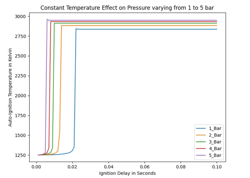
From the above plot it can be seen that increase pressure will surely reduce the auto-ignition temperature for fuel & air mixture. Ignition delay time is reduced for the higher pressure fuel and air mixtures. Reduced ignition delay will provide better burning of fuel and less emission from engine exhaust. The actual time of auto-ignition at different pressure is given as:
For 1 bar pressure = 21 miliseconds
For 2 bar pressure = 13 miliseconds
For 3 bar pressure = 09 miliseconds
For 4 bar pressure = 07 miliseconds
For 5 bar pressure = 04 miliseconds
Resutls Part 2: -
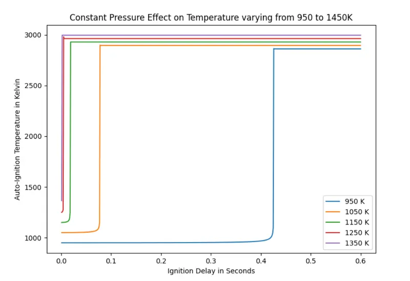
From above plot, it can be seen that increase in the fuel air mixture temperature reduce the ignition delay significantly. The actual auto-ignition time for various temperature are given as:
For 950 Kelvin = 425 miliseconds
For 1050 Kelvin = 77 miliseconds
For 1150 Kelvin = 19 miliseconds
For 1250 Kelvin = 6 miliseconds
For 1350 Kelvin = 3 miliseconds
Coding Approach for Part 3 & 4: -
In part three the molar concentrations of the species which are involve in the combustion has been calculated and plotted along with respect to time. For this approach two temperature are selected which are 500 k and 1000 K. In this code two solution arrray are created for each of the temperature range and species are determined. Figure has been created with subplot of 3 rows which shows the species molar concentration of H2O, O2 and OH. The part four is just a replica of part two in which only two temeprature has been used to calculate the auto-ignition temperature and its observation has been done. The code for part 3 and 4 is shown below:
Part 3: -
"""
Determining Auto Ignition Temperature Using Cantera
Part 3: - Calculating Rate of Change of Molar Concentration of 'H2O, O2, OH'
When Temperature is 1000 K and 500 K at 5 Bar pressure
Simulation time is 10 seconds
Properties of Fuel: CH4:1 moles, O2: 2 moles and N2: 7.52 moles
Command: states.X[:,gas.species_index('species')]
Code Written by: Shubham Chaudhari
Skill Lync Challenge Week 7
"""
import sys
import cantera as ct
import matplotlib.pyplot as plt
import numpy as np

# Creation of Gas object
gas = ct.Solution('gri30.xml')
T = [500,1000]                          # specification of temperature
P = 5*101325                            # Specification of Pressure
auto_igni_T = []                        # Defining list of time

a = 0
j = 0
for j in range(2):
    gas.TPX = T[j],P,{'CH4':1,'O2':2,'N2':7.52}
    r = ct.IdealGasReactor(gas)
    sim = ct.ReactorNet([r])
    time = 0.0
    states = ct.SolutionArray(gas,extra = ['time_in_ms','t'])
    states2 = ct.SolutionArray(gas,extra = ['time_in_ms','t'])

    if j == 0:
        for i in range (10000):
            time += 1e-3
            sim.advance(time)
            states.append(r.thermo.state,time_in_ms = time*1e3, t=time)

        f = plt.figure(1)
        plt.subplot(3,1,1)
        plt.plot(states.t,states.X[:,gas.species_index('H2O')],color = 'blue')
        plt.ylabel(['H2O'])
        plt.title('Molar Concentration of H2O')
        plt.legend(['T = 500K'])
        f.set_figwidth(10)
        f.set_figheight(17)

        plt.figure(1)
        plt.subplot(3,1,2)
        plt.plot(states.t,states.X[:,gas.species_index('O2')],color = 'blue')
        plt.ylabel(['O2'])
        plt.title('Molar Concentration of O2')
        plt.legend(['T = 500K'])

        plt.figure(1)
        plt.subplot(3,1,3)
        plt.plot(states.t,states.X[:,gas.species_index('OH')],color = 'blue')
        plt.ylabel(['OH'])
        plt.title('Molar Concentration of OH')
        plt.legend(['T = 500K'])


    if j == 1:
        for i in range (10000):
            time += 1e-3
            sim.advance(time)
            states.append(r.thermo.state,time_in_ms = time*1e3, t=time)

        f = plt.figure(2)
        plt.subplot(3,1,1)
        plt.plot(states.t,states.X[:,gas.species_index('H2O')],color = 'red')
        plt.ylabel(['H2O'])
        plt.title('Molar Concentration of H2O')
        plt.legend(['T = 1000K'])
        f.set_figwidth(10)
        f.set_figheight(17)

        plt.figure(2)
        plt.subplot(3,1,2)
        plt.plot(states.t,states.X[:,gas.species_index('O2')],color = 'red')
        plt.ylabel(['O2'])
        plt.title('Molar Concentration of O2')
        plt.legend(['T = 1000K'])

        plt.figure(2)
        plt.subplot(3,1,3)
        plt.plot(states.t,states.X[:,gas.species_index('OH')],color = 'red')
        plt.ylabel(['OH'])
        plt.title('Molar Concentration of OH')
        plt.legend(['T = 1000K'])

plt.show()
Part 4: -
"""
Determining Auto Ignition Temperature Using Cantera
Part 4: - Calculating Auto Ignition Time of Methane at Constant Pressure of 5 Bar
with 500 K and 1000 K
Simulation time is 10 seconds
Properties of Fuel: CH4:1 moles, O2: 2 moles and N2: 7.52 moles
Code Written by: Shubham Chaudhari
Skill Lync Challenge Week 7
"""
import sys
import cantera as ct
import matplotlib.pyplot as plt
import numpy as np

# Creation of Gas object
gas = ct.Solution('gri30.xml')
T = [500,1000]                          # specification of temperature
P = 5*101325                            # Specification of Pressure
time = np.zeros(5)                      # Defining list of time

# Different Pressure variable for saving auto ignition time
states_T1 = []
states_T2 = []


for i in range(2):
    gas.TPX = T[i], P, {'CH4':1,'O2':2,'N2':7.52}
    r = ct.IdealGasReactor(gas)
    sim = ct.ReactorNet([r])
    states = ct.SolutionArray(gas,extra=['time_in_ms','t'])

    for j in range(600):
        time[i] += 1e-3
        sim.advance(time[i])
        states.append(r.thermo.state, time_in_ms = time[i]*1e3, t = time[i])

    # Use of Condition for storing different value of pressure
    if i == 0:
        states_T1 = states.T

    if i == 1:
        states_T2 = states.T

f = plt.figure(1)
plt.subplot(2,1,1)
plt.plot(states.t, states_T1)
plt.title('Behaviour of Auto-Ignition Temperature at 500K and 5 Bar Pressure')
plt.ylabel('Auto-Ignition Temperature in Kelvin')
plt.legend(['500 K'])
plt.figure(1)
plt.subplot(2,1,2)
plt.plot(states.t, states_T2)
plt.title('Behaviour of Auto-Ignition Temperature at 1000K and 5 Bar Pressure')
plt.xlabel('Ignition Delay in Seconds')
plt.ylabel('Auto-Ignition Temperature in Kelvin')
plt.legend(['1000 K'])
f.set_figwidth(10)
f.set_figheight(17)
plt.show()
Results Part 3: -
Rate of Change of Molar Concentration of Species at 500 Kelvin and 5 Bar pressure
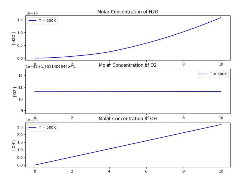
In above plot it can be seen that the molar concentration of all the species are unrealistic at the lower temperature because no ignition has been done. All the value of molar concentration are negligible.
Rate of Change of Molar Concentration of Species at 1000 Kelvin and 5 Bar pressure
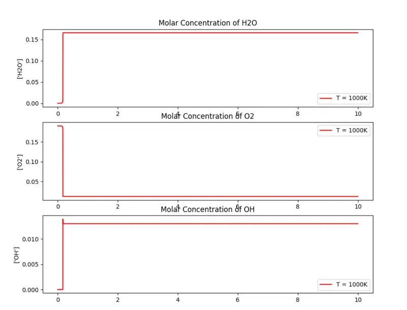
In above plot it is clearly visible that after the few miliseconds the molar concentration of all species are in considerable range. It can be seen that the combustion has been occure because the concentration of O2 is decreased and increase of OH concentration.
Result Part 4: -
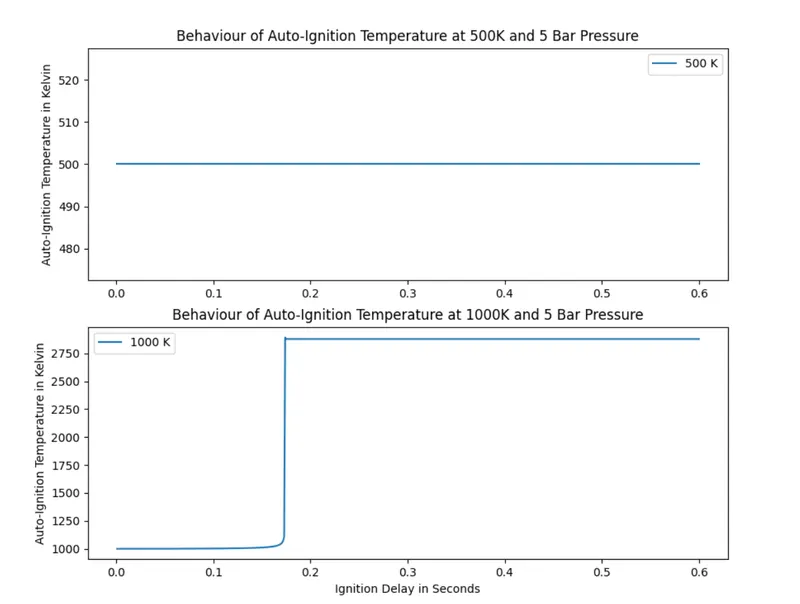
From above plot it can be seen that, for 500 kelvin and 5 bar pressure there is no combustion is occured for air-fuel mixture whereas for 1000 kelvin temperature the ignition delay is taking place after 17 miliseconds which tells that this is suitable temperature for auto-ignition of methane in constant volume chamber.