Week 6 - CHT Analysis on a Graphics card

Aim: - To perform conjugate heat transfer analysis of a Graphics Card setup.

Objective: -

• To study the importance of conjugate heat transfer.
• To pre-processes the geometry for CHT analysis using space-claim.
• To mesh the geometry appropriately and explain the reason for choosing particular settings.
• To check the quality of mesh and perform mesh independent test for correct mesh size.
• To select the material for graphics card and evaluate volume heat flux value for processor.
• To setup the conjugate heat transfer simulation for the problem.
• To post-processes the results based on convergence and heat transfer coefficient.
• To vary the inlet velocity and compare the results based on observation.

Introduction: -

Conjugate heat transfer simulation are mostly used where the temperature on the solid with respect to fluid flow are carried out. The most important part of the simulation is to setup the both flow field and energy equation to solve simultaneously. Conjugate heat transfer is based on the natural convection where fluid motion is generated due to density difference and in case of forced convection it is generated due to the pressure difference in flow field. In most of the application of heat transfer problem, conjugate heat transfer is used when user need to confirm that solid temperature should not go beyond material melting temperatures also the temperature of solid should not be constant for most of time. In this problem where we are going to simulate the heat transfer of the graphics card where graphics processor is the main heating part in the assembly. The below image shows the parts of graphics card assembly.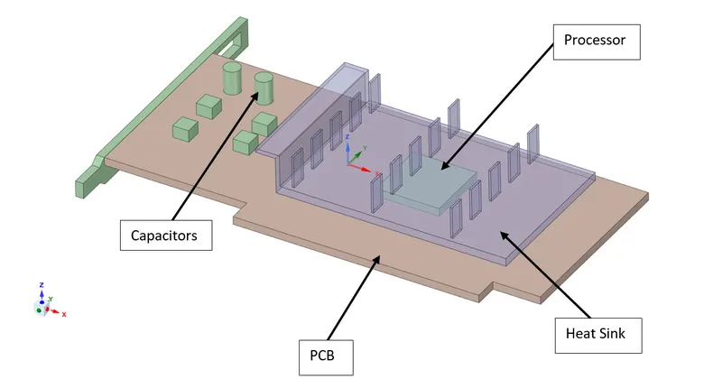

In above figure we can see the processor is directly mounted over PCB and on it there is heat sink provided which will be having more surface area to dissipate the heat to air via natural or forced convection. In actual graphics card there is the exhaust fan is provided to lower the temperature of processor and maintain it at certain operating temperature range. The PCB is the component where all the connection has been provided from processor to the other unit of graphics card, it is also important to maintain the temperature of PCB in any case because it has carved the lines which can be get diminished or erased if the temperature goes beyond the rated temperature. The wattage of the graphics card is depending on the how much number of pins are provided. The material of graphics card is mostly copper or gold which high thermal conductive materials. Gold is seen at high rated and costly graphics card. The use of conjugate heat transfer analysis is to make sure that temperature should not go beyond the working temperature of heat sink and PCB. The most mistake done by the user in case of conjugate heat transfer analysis of graphics card or any other electronic device in which LED or processor are used as main heat creating parts is that they directly provide the amount of heat flux to the processor or LED which utterly wrong. If we know the process how processor is installed on the graphics card, we can see that there is some application paste which is called thermal paste inserted before processor mounted on PCB and heat sink placed on processor. This thermal paste has thermal conductivity properties and need to be included in the simulation for actual simulation results. This paste is also called substrate in the most of the headlight applications where LED are used.

Simulation Methodology: -

The methodology which is used in this simulation is to first predict the right mesh size for the model by performing mesh independent test and then later on use the different velocity rate to compare the results of temperature generated by processor to heat transfer coefficient achieved during simulation. The simulation is divided in seven different cases in which first four cases are used to check mesh independency and later one are used to simulate with different velocity numbers. The cases are given as below:

Case 1: - CHT analysis of graphics card with baseline mesh setup and with 1m/s velocity.

Case 2: - CHT analysis of graphics card with refined mesh setup and with 1m/s velocity.

Case 3: - CHT analysis of graphics card with further refined mesh setup with 1m/s velocity.

Case 4: - CHT analysis of graphics card with last refined mesh setup.

Case 5: - CHT analysis of graphics card with 2m/s velocity value.

Case6: - CHT analysis of graphics card with 3.5m/s velocity value.

Case 7: - CHT analysis of graphics card with 5m/s velocity value.

For each of the cases the results are provided with temperature and heat transfer coefficient value. The mesh independent test is carried by looking at the temperature, residuals and standard deviation graphs. The methodology which is used for the simulation is same as used for the previous case of exhaust manifold simulation, but here we are not calculating the heat transfer coefficient for the setup. In this simulation we are not providing any convection heat transfer boundary conditions instead of it as it is an external flow simulation the air velocity is taking care for convection boundary condition itself. In most of the electronic related simulation the flow conditions are external and somewhat internal. In case of external flow simulation, it is important to provide the fluid domain in which fluid has to be pass, and area of interest is placed in that domain which we called as enclosure. After providing enclosure it is important to conformal mesh between the enclosure and the part on which temperature has to be recorded. Having conformal mesh is an option for the user as inconformal mesh also can provide similar results. ANSYS meshing has the contact group which is responsible for delivery of result from one contact pair to another. The only thing which need to be taken care of is there should be no possible overlapping faces in the model this will make life difficult during the simulation. Hence it is better to use the conformal mesh for lower complexity problems. The other disadvantage of conformal mesh is that we need to always go with minimum mesh size to capture the results in better response. Providing same mesh size for all the component increase the computational time for simulation and put severe risk on the computer. The conformal mesh in ANSYS can be create by using share topology option in space-claim. This allow the faces and edges of geometry to seen as only one. After creating the conformal mesh, it is important to provide the name of boundary conditions in workbench as it will carry forward the information to the FLUENT as inflow or outflow boundary conditions depending upon setup of model.

As simulation is external flow and temperature has to be evaluate both turbulence and energy equations has to be checked for the problem. The use of K-omega SST model for the simulation is selected because it can provide the advantage of K-epsilon with K-omega model to capture the boundary layer information. For the whole simulation it is very important to know which is solid domain and fluid domain respectively. Assigning the material is one part but important part is where the governing equation are to be solved. If user makes the mistake in determining the proper domain where heat transfer takes place, then he has to do the process entirely again which is time consuming. After assigning the material and selecting proper domain information to the solid and liquid it is necessary to provide the boundary condition as stated in workbench. The velocity inlet and pressure outlet are the main boundary conditions are used in this simulation with inlet temperature of 25℃ and outlet temperature as same of inlet one. The pressure-velocity coupling which is used for simulation is SIMPLE and pressure coupling is linked with PRESTO as standard pressure discretization can give rise to incorrect velocity near the wall area of graphics card. This same setup has been used for all the simulation and each simulation is run for 500 iterations in which all the setup has got their convergence.

Geometry Pre-Processing: -

The geometry comprises of most of the main components of the graphics card provided in the problem. The pre-processing of the geometry is takes place in the space-claim where all the changes has been made to geometry. The main changes in the geometry is to create the substrate from the processor. First it is required to create two new components in the existing graphics card assembly. Then making processor geometry as active component and hiding every other component in the assembly for better visibility. Creating the plane on top of the processor face and moving it downward by 0.15mm, using split body option in space-claim to split the processor in two solid. The solid geometry which was created can be directly move to the substrate component by drag and drop from the components tree. Similarly, another solid need to be created in the bottom face of the geometry in same way and need to be drop in the substrate 2 component. After creating the two substrate in bottom and top of the processor the geometry will look like:

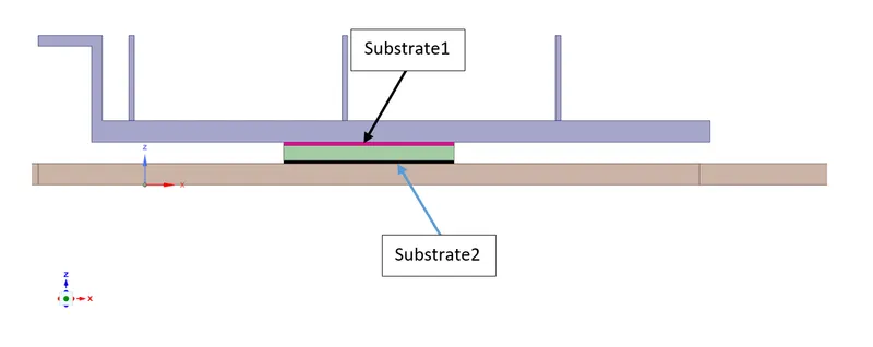
The work of substrate is to not expose hot temperature generated in the processor directly to the PCB and heat sink in the graphics card. The substrate is again come up with layer of copper on top of it but this methodology is not used in the graphics card electronic components besides it used in LED lamps of automobile.

After creating substrate in the geometry, to facilitate the flow over the graphics card assembly the enclosure has to be created which is already present in the geometry file. The only thing need to be done is to make sure all the faces and edges are shared with enclosure geometry. This can be done by using share topology tool in space-claim. After performing the share topology method, the geometry will look like:

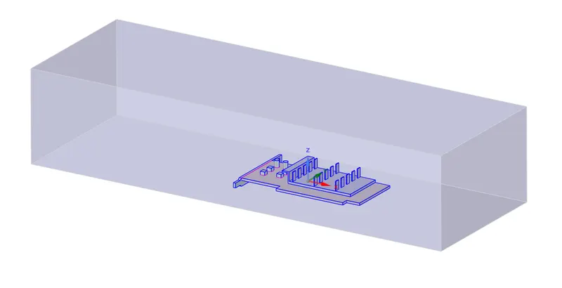
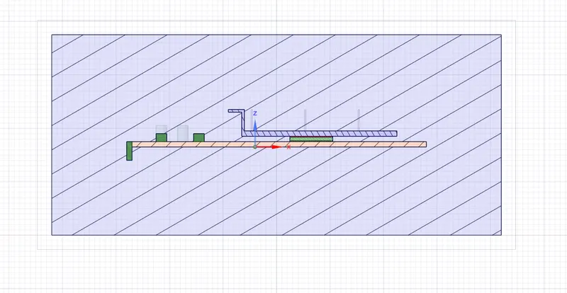
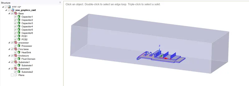
After the completing the share topology tool it is important to check the available interference in the model. Interference in the model will create abrupt mesh in the geometry which will be ill-treated in the simulation. Before moving in the workbench it is better practice to rename each of the component present in the assembly according to its working name. It will give better understanding to user while meshing and selecting the walls and other interior for solver setup and post-processing. After providing the input to names the final pre-processed geometry will look like:

Meshing: -

The meshing of such geometry are needed to be done with respect to the application of simulation and determining the best suited mesh for the problem. As the geometry is bit more complex with respect to sharing the faces and edges with enclosure it is required to have better local mesh control over global. User can use both of the mesh control but in such case were parts are more, then conjunction of global mesh over local mesh control have more impact. The meshing is an art, every individual can bring his own mesh with his own parameter and clarification. For meshing any geometry, it is important to notice what is least minimum size of edge is present in the geometry. This length of edge can be used as mesh size for the whole geometry but it will create more number element in the process. Hence use of global mesh size control and local mesh size control are important in such scenario.

The default mesh method used in ANSYS workbench are patch conforming and sweeping. Patch conforming is used for tetrahedral mesh and sweeping is used for hexahedral mesh type. Hence when any geometry which resemble the both normal shape and complex shape the ANSYS workbench mesh algorithm meshes normal shape geometry (e.g. circle, rectangle, square) into hexahedral mesh whereas complex geometry in tetrahedral mesh providing advantage of both. In our case of geometry, we have similar type of application where we have processor and capacitors as normal shape geometry and heat sink as complex geometry. Creating the baseline mesh without any intervention in global setting and local mesh setting will provide coarse mesh at bigger geometry and maintaining proximity features in the smaller geometry. After creating the baseline mesh, the mesh will look like:

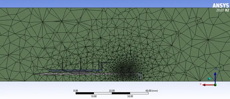
As we can see from the above figure that smaller mesh size elements are created near the capacitors and as we move away the mesh algorithm will provide bigger mesh elements. Now the question arises which elements are better either hexahedral or tetrahedral elements. For the simulation if complex geometry is present it is better to go with tetrahedral elements because they are easy to generate and less time consuming and will provide efficient results at the end, whereas hexahedral mesh type is used with most 2D simulation where geometry is quite easy and can be degraded in number of simple geometry. Hexahedral mesh will provide better result accuracy in response to tetrahedral mesh but creating former element are quite time consuming and have lower mesh quality.

If we run the simulation on the baseline mesh it will never converge because the number of element created are very small and for conjugate heat transfer analysis, it is always recommended that very fine mesh size is required at the heat source or it will diverge the solution in most probable time. Hence it is required to lower the mesh size for the baseline simulation.

Baseline Mesh Setup

The original mesh setup what discussed earlier is not enough to provide the good simulation hence it is required to lower the mesh size for the better simulation. In case of baseline mesh setup only the global mesh controls are used because of its simplicity and use of shape function in the meshing algorithm. The advance shape function in meshing algorithm are curvature and proximity where curvature is used with round shape object and proximity is used in object with sharp steps. If the geometry comprises of both then user can use both of the advance shape function. In this case both shape functions are used according to the size of element required. The mesh setting parameter are used in the baseline mesh setup are given as:

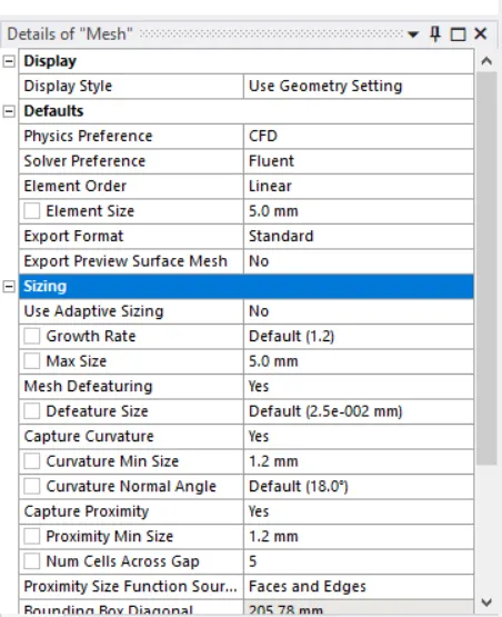
In above figure it was seen that, the mesh is using both size function parameter which are proximity and curvature in which curvature minimum size and proximity minimum size are kept same to get structured mesh at all platform which is 1.2mm and maximum size of element which was default of 10.23mm in first mesh setting was changed to 5mm. After application of this setting parameter the mesh will look like:

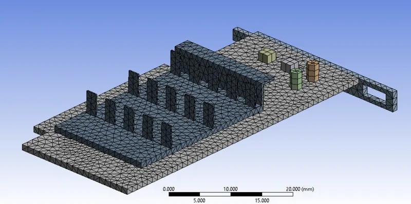
This is the mesh for the graphics card components with proximity and curvature minimum size of 1.2mm. It can be seen that the mesh is quite coarse at all the places and as discuss earlier for the normal shape geometry it can see that hexahedral mesh elements are present whereas for complex shape geometry meshing algorithm provides tetrahedral elements. The section view of baseline mesh is shown below:

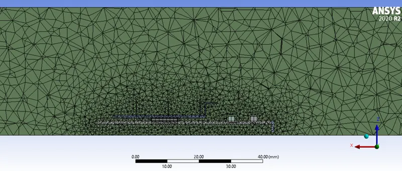
In section view the growth rate parameter which is 1.2 default is used by meshing algorithm to scatter the element when going far from the less mesh size elements. The total number of element create in baseline mesh setup is 154398. It is important to check the mesh element quality as it will affect the solution accuracy. In baseline mesh setup the skewness element quality is checked only as it is vice-versa to element quality in ANSYS workbench. The graph of skewness element quality is shown below:

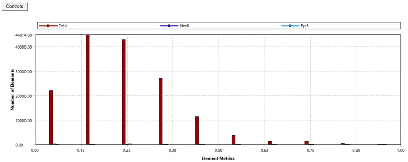
There are only 4-10 elements with the skewness of 0.96 hence can be allowed in the simulation as it will not drastically change the accuracy of the solution. For element quality setup if 80-85% of element are in best conditions and remaining elements are bad condition it is possible to move up for the simulation still it will be remembered that location of bad element should be taken into considerations.

FLUENT SETUP: -

When the flow occurs over a heated body it carries the heat with it, this is called as natural convection. In this case of conjugate heat transfer according to the application the flow may be natural or forced. The FLUENT setup need to have the both fluid flow and heat transfer at the same place to solve the heat transport equation with momentum and continuity equations. Problem has to be solve with steady state application and energy equation as checked for the solution. For some cases where energy equation can be turned on after solving fluid flow equation this provide better option to energy equation to solve with great conversion.

For fluid flow equation, the turbulence equation which has been used for simulation is K-omega SST model. K-omega SST model are used where highly accurate resolution of boundary layers is critical such as application involving flow separation or finely resolved heat transfer profile. SST model is a hybrid two equation model that combines the advantage of both k-omega and k-epsilon. The K-omega and K-epsilon model are blended in a such way that in SST that near the wall it use K-omega and in freestream it uses K-epsilon. The wall treatment is considering as standard as there is no need for calculating shear stress near the walls. The next thing is in the simulation is material selection.

• Material Selection

The material which are used in the simulation are mostly similar to the real life application.

1. PCB

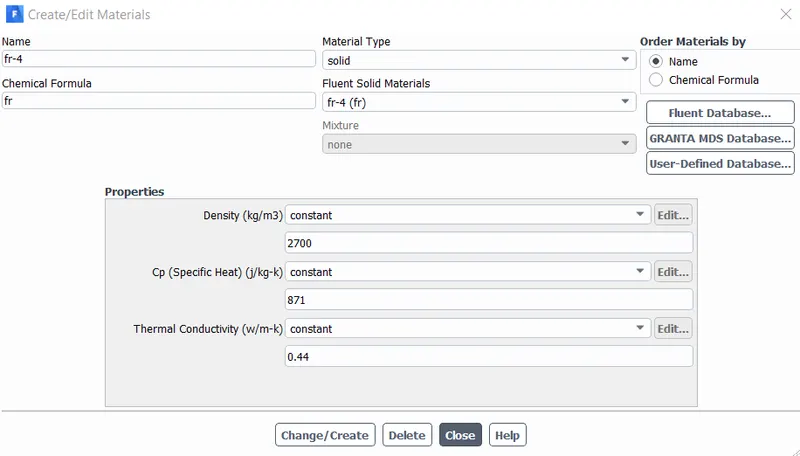
The base which is PCB of graphics card is consider as FR4 material. FR4 material is commonly used in the industry for printed circuit boards and it is a composite material made up of woven fiberglass cloth with an epoxy resin and it is flame resistance. The FR is stand for Flame retardant. The property of FR4 in FLUENT is given as:

2. Capacitors

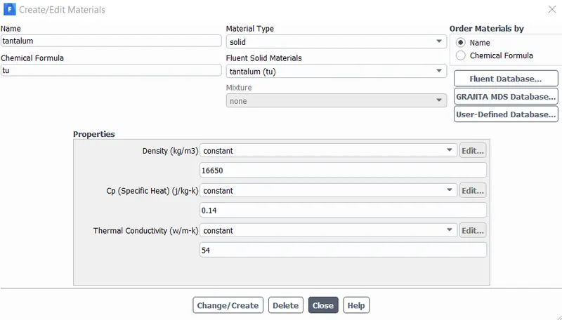
The capacitors in the graphics card is made of tantalum material. Tantalum is mostly used as alloy with aluminum to add the high strength, ductility and high melting point. The electrolyte capacitors are having more than half of tantalum present in it. The material properties of tantalum are given below:

3. Processor

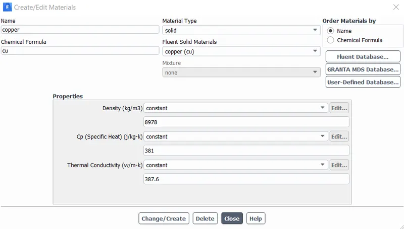
The processor of the graphics card is made of millions of transistor and capacitors. This is very difficult to put inside the simulation as those are very minute. Hence we are considering the processor as the copper material having high thermal conductivity. The material properties for processor are given below:

4. Substrate

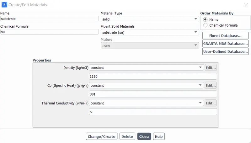
As state earlier the substrate is the paste of thermal resistance material and pasted on and below of the processor before mounting. It is applied on the heat sink also. It acts as the resistive shield between processor and heat sink or PCB. The material properties of substrate are given below:

5. Heat sink

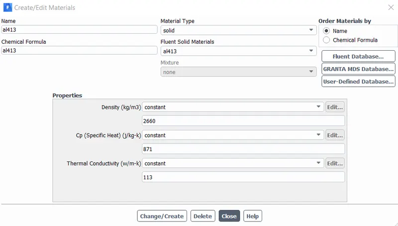
The heat sinks are made up of common material alloy of aluminum. The AI413 is most suitable and popular aluminum alloy used for the heat sink application for most of the electronic components. The material properties for heat sink are given below:

These materials are provided to geometry in the cell zone conditions. In the cell zone condition there is option of providing the source term which will act as heat flux condition. The calculation of volume heat flux is depending on the volume of the component which is producing heat and wattage of the component. The graphics card processor is bigger in most of the application whereas the dimension of processor is bit smaller which are provided. Hence using the actual wattage of the real time graphics card is not going to provide real world simulation results. The volumetric area of the processor after creating two substrates from it is around 45mm³. The wattage of the processor is considering as 5 watts, then the total heat flux provided to the processor is calculated by:

`Heat flux=5/(4.5e^(-8) )= 111111111.11 W/m^3`

This value of volume heat flux is provided to the processor present in the assembly. It can be done by selecting the processor in cell zone condition and after applying copper as material there is the option of source term which need to be check and in source term there is option of value which need to be provided where user has to select as constant to provide the value. The power wattage which has been consider for the problem is mostly seen in the 6 pin graphics card which are now absolute in use in electronics industry. If we consider Nvidia GTX 1050 graphics card which is used for gaming purpose its processor uses 75 watts as the input and maximum temperature attained by the graphics card processor is 97℃. This value can’t be use for this simulation because the dimension of processor in GTX 1050 are way bigger than what geometry of processor is provided in the problem.

• Boundary Conditions

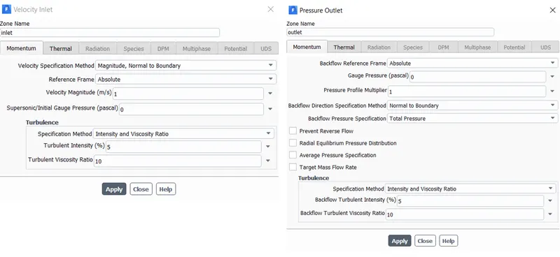
The simulation has only three boundary condition which are inlet, outlet and symmetry as wall function. For the first four simulation case the inlet boundary condition is same in all respect which is 1m/s and the inlet temperature is 25℃. The outlet boundary condition is selected as pressure-outlet with outlet temperature of 25℃. The rest of the walls of enclosure are selected as symmetry. The boundary condition as shown below:

• Solver Setup

The conjugate heat transfer problems are mostly steady state in nature where user need to find the results at the start and at the end of the simulation. The solver is pressure based because of low Reynolds number. There is one implication in the simulation regarding working fluid as air. The density of air for most of the simulation is kept constant but for the conjugate heat transfer it can be change to incompressible ideal gas because of the air near the hot object get heated. Increase in the temperature of the air could rise to change of density of air hence the results of the simulation may not be correct with operating density option in FLUENT. Hence for the most of the case where temperature is rise is more the air is treated as incompressible ideal gas where density effect due to temperature are neglected is used. For this case air is treated as constant at density there is no need to use pressure is treated as PRESTO and can be use STANDARD function for calculation pressure term in transport governing equation. For better convergence the calculation of turbulent kinetic energy can be treated as second order rather than first order. It can be said that use of under relaxation factor to achieve convergence can be used by varying energy relaxation factor to 0.9 or 0.95. This under relaxation factor can be only used when the skewness of the elements is out of reach from the limit. For simulation the under relaxation factors are consider constant and default.

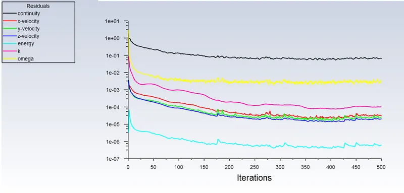
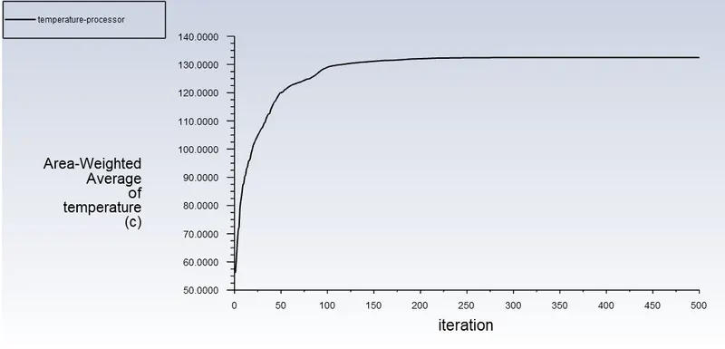
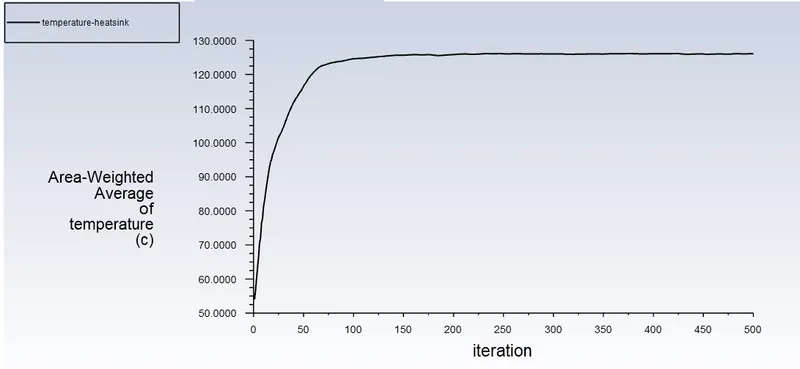
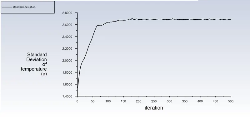
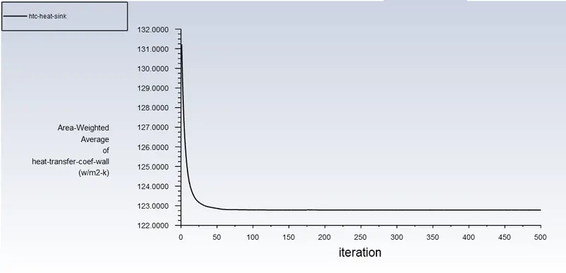
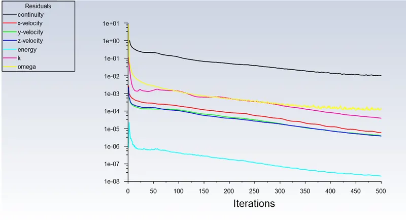
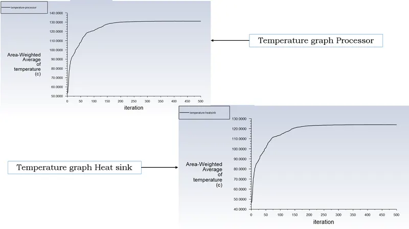
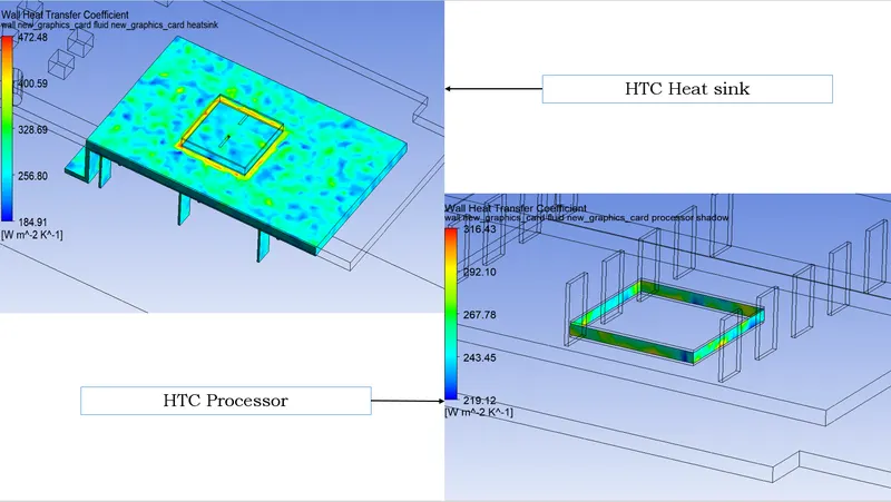
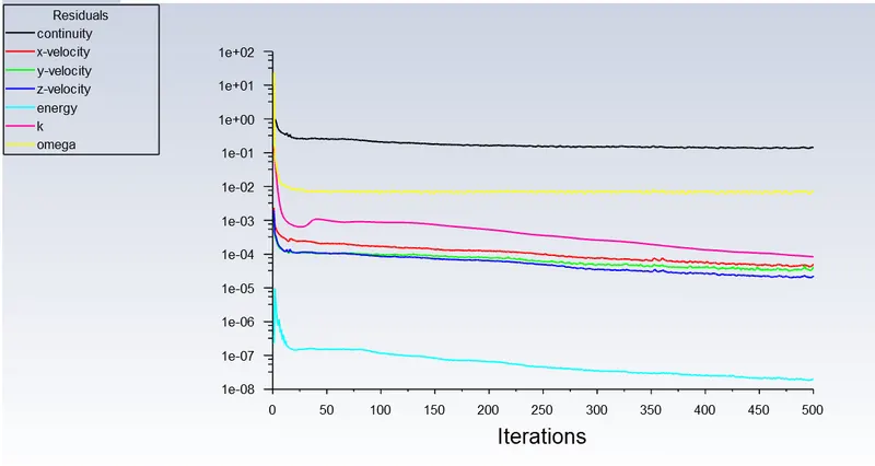
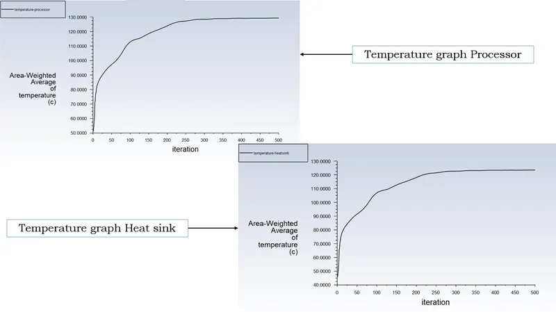
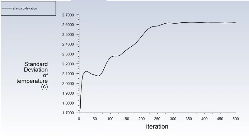
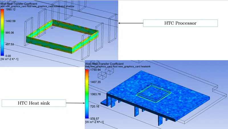
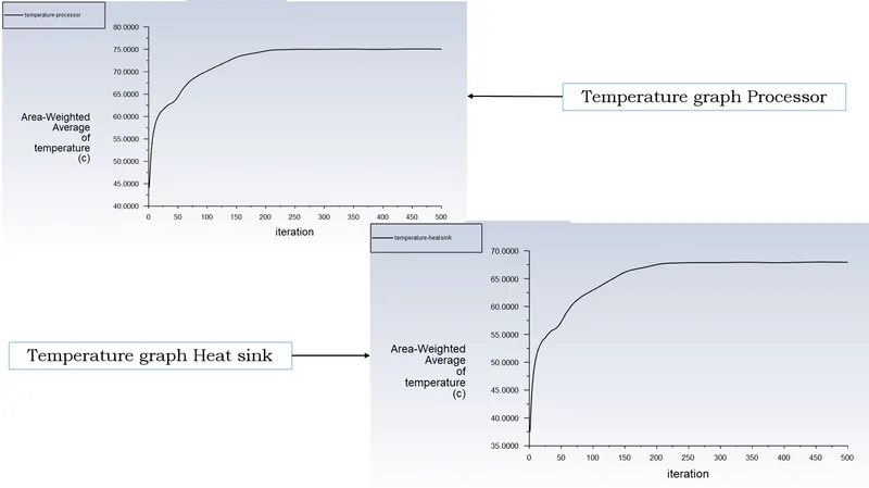
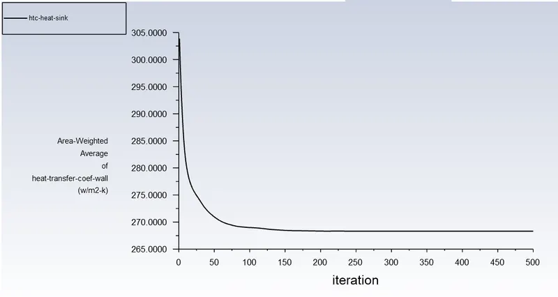
To check the convergence of the problem rather than rely on the residual it is need to create some graph which tell about when temperature steady state level is achieved. The temperature of processor and heat sink are tracked while the solution iteration are being computed. The standard deviation of temperature is also used to check the difference in between mesh independent test and the animation of temperature is created on the heat sink to further check the discontinuities in solution while iterating. The heat transfer coefficient graph is created on the heat sink. To perform the post processing in the FLUENT result post processor the data file quantities are written before start the iteration in which all the results regarding temperature and heat transfer coefficient are computed and forward to the post-processor.

CASE 1: - BASELINE MESH SETUP RESULTS

1) Residual

2) Temperature plot on processor

3) Temperature plot on heat sink

4) Standard deviation of temperature

5) Heat transfer coefficient

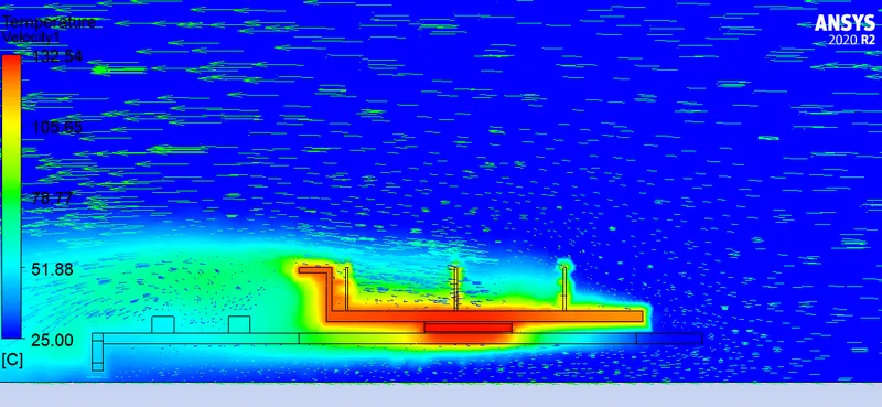
6) Velocity Vector and Temperature contour

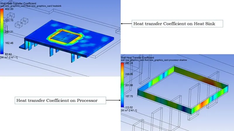
7) Heat transfer coefficient

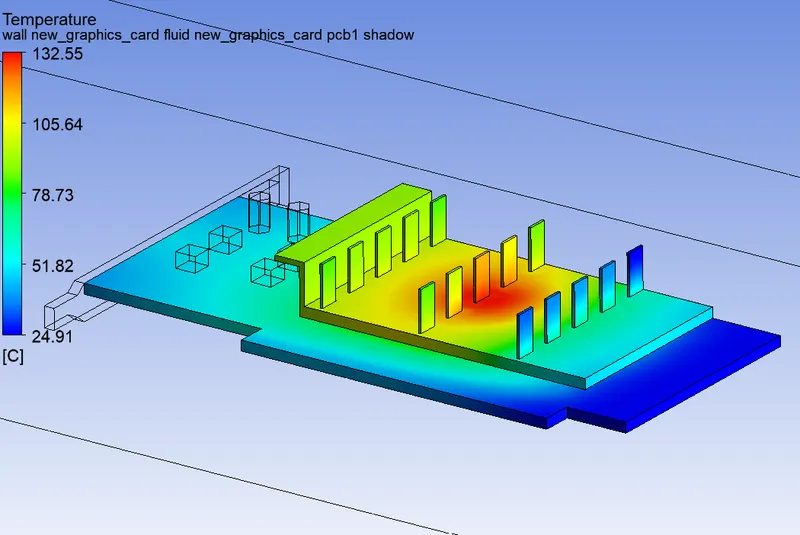
8) Temperature contour on heat sink

CASE 2: - MESH INDEPENDECY TEST 1

From the result of first case we can see contours are very well created and balanced hence can be say that whatever mesh has created is having better quality to provide the results. But this results are not at par with simulation. To get the accurate and refined results it is important to reduce the size of mesh. In first mesh independency test the minimum size of the size function proximity and curvature is 0.75mm and the maximum element size is around 5mm. The total amount of element created in the mesh is 392096. The mesh for the first independency test 1 is shown below:

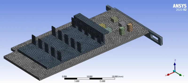
In above figure it can be seen that the amount of element in components of graphics card are increased as compare to the baseline mesh. It is possible to only create element near the processor and capacitors in the assembly but making it crowded with small element put the effect on the major body element size while having the conformal mesh. Hence it is better practice to go with size function in global control to vary the element size. The section view of the mesh is shown below:

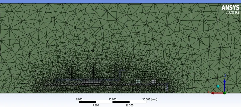
RESULTS: - MESH INDEPENDENCY TEST 1

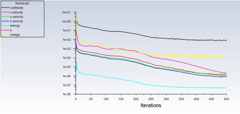
1) Residual

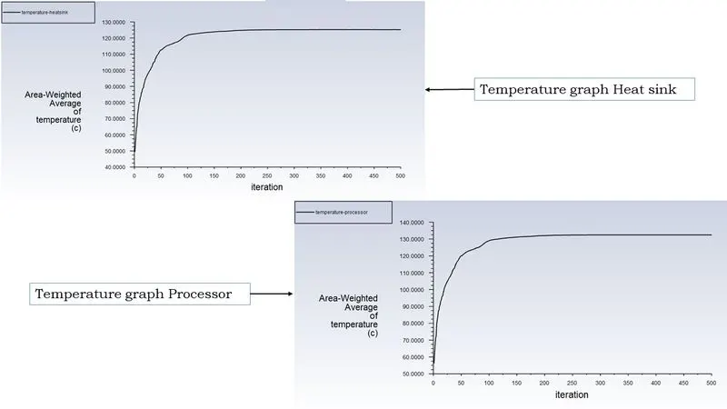
2) Temperature graph

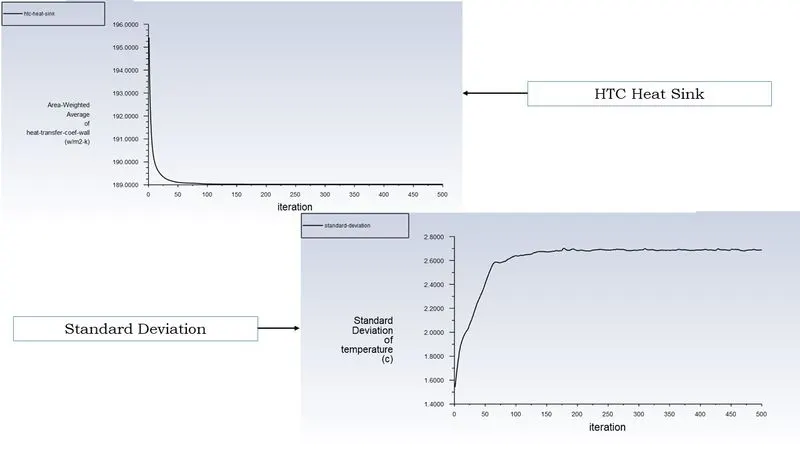
3) HTC and SD

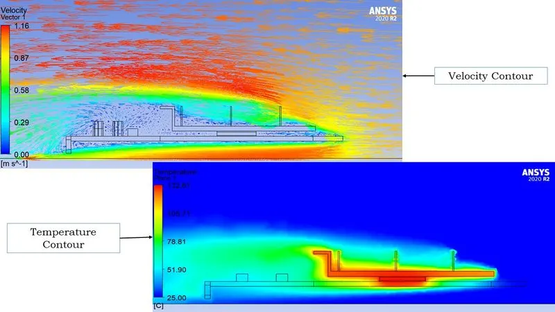
4) Velocity and Temperature contour

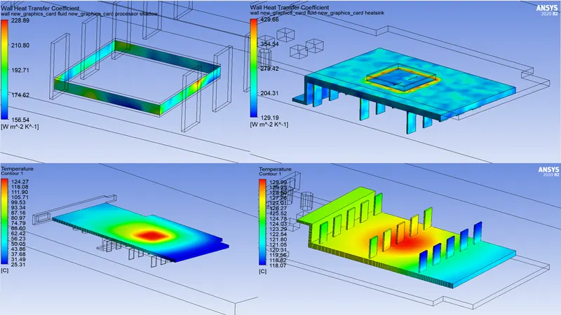
5) Hotspot and HTC

CASE 3: - MESH INDEPENDECY TEST 2

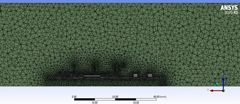
From the two mesh independency test it was seen that temperature is lowered as mesh size increased. The standard deviation seems to be similar but drop in size with minimum range. To further check for accuracy of the solution it required to lower the size of mesh. For this test the minimum size of the mesh is consider as 0.5mm and maximum size of the mesh is considering as 2.5mm. The total number of element created in the second test is 1008137. The mesh of the component is shown as:

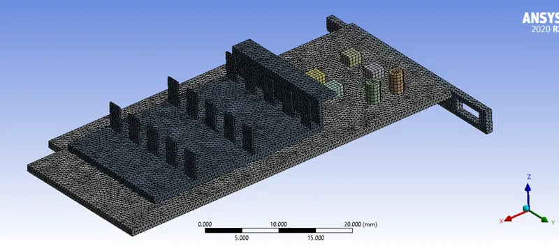
From above it can be seen that the mesh element in all area of component in assembly are mesh with given mesh size. The section view of the total mesh is shown below:

RESULTS: - MESH INDEPENDENCY TEST 2

1) Residual

2) Temperature graph

3) HTC and SD

4) Heat transfer coefficient

5) Hotspot in model

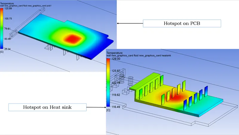
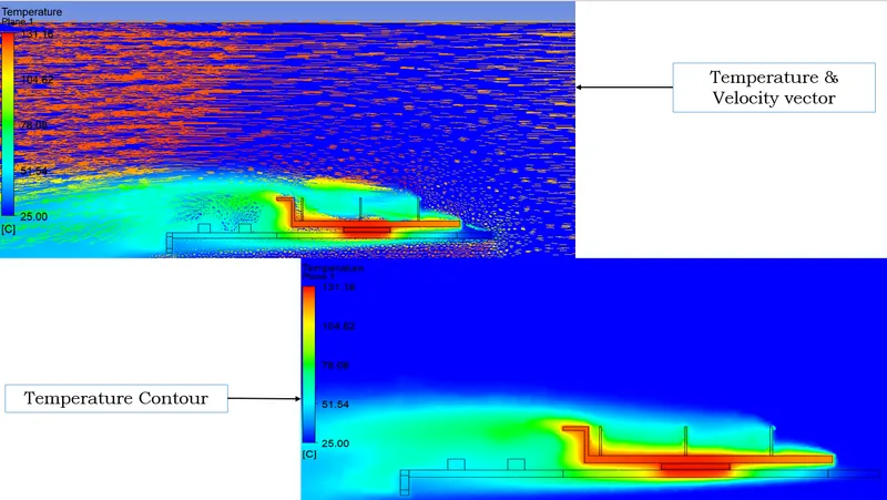
6) Velocity Vector and Temperature contour

CASE 4: - MESH INDEPENDECY TEST 3

Form the previous simulation result the temperature is drop by just 2℃. While designing any new component the tolerance of 1 unit is important. Hence it was necessary to lower the size of the mesh to get more refined results. It seems that lowering the meshing size by half will get to the minimum edge length of assembly. Lowering size of element below the minimum edge of the assembly will create huge number of element which will put the more stress on the resource. For this case the minimum size of the element is 0.25mm which is minimum edge size in the assembly. The maximum size is lowered to 1.5mm. The total number of element created in the case four is 4476328. The mesh for case four is shown below:

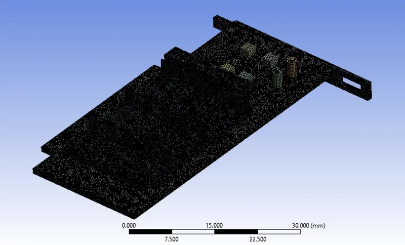
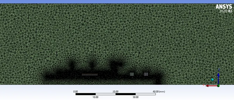
From above image it can be seen that the mesh size way too much lower and created more than 40 lakhs of elements. The section view of mesh is shown below:

RESULTS: - MESH INDEPENDENCY TEST 3

1) Residual

2) Temperature graph

3) Standard deviation

4) Heat transfer coefficient contour

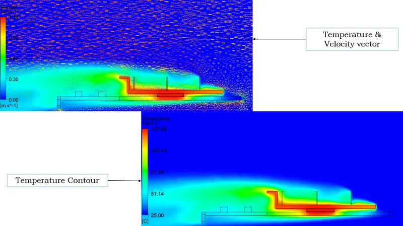
5) Velocity and Temperature contour

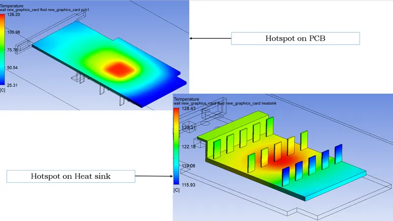
6) Hotspot in Assembly

MESH INDEPENDENCT TEST TABLE

Parameters	Avg Temperature at Processor ℃	Avg Temperature at Heat sink ℃	Standard deviation of Temperature	Maximum Temperature at Heat sink ℃
Case 1	132.41	125.14	2.73	132.55
Case 2	132.46	125.20	2.73	129.99
Case 3	131.00	123.86	2.62	129.00
Case 4	130.95	123.24	2.617	128.43

CASE 5: - Conjugate heat transfer analysis with velocity 2m/s

In above four cases of simulation only the mesh independency was checked with constant velocity of 1m/s. It was found that using case 4 mesh size will take longer time to provide the results as compared to case 3. The difference of results between the two are not bigger and can be used for rest of the simulation were velocity is varied. The mesh with minimum size of element of 0.5mm and maximum size of 2.5mm is used to case five where the velocity is increased from 1m/s to 2m/s. The objective of this simulation is to find out the comparison between the conjugate heat transfer analysis with different velocities. The whole setup of the simulation is similar the only thing which has been changed is velocity value in inlet velocity boundary condition. The results of the case five are given below:

RESULTS: - CASE 5 (VELOCITY = 2 M/S)

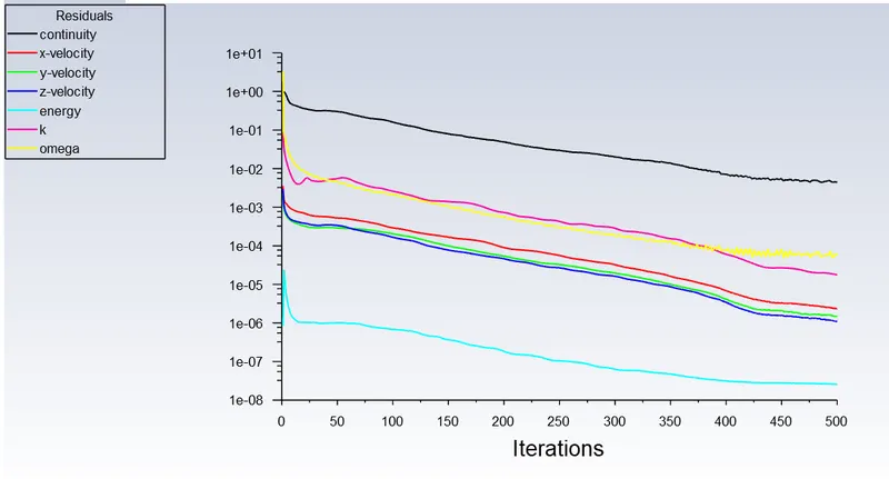
1) Residual

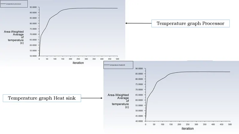
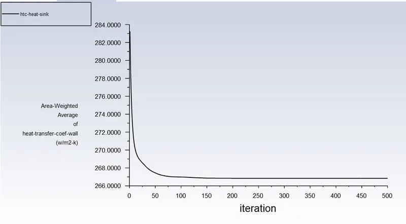
2) Temperature graph

3) Heat Transfer coefficient

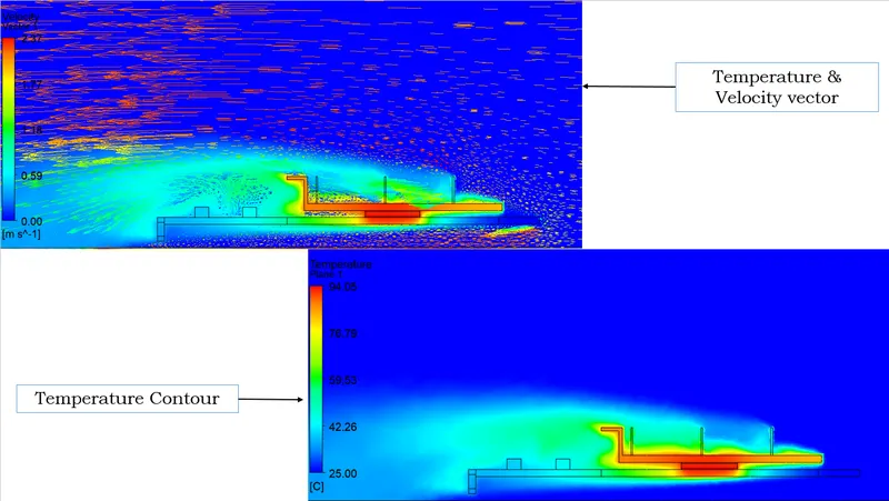
4) Velocity and Temperature contour

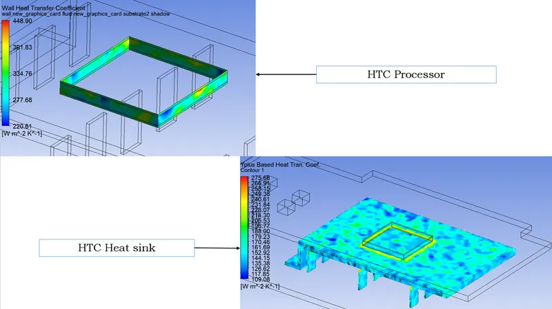
5) Heat transfer coefficient contour

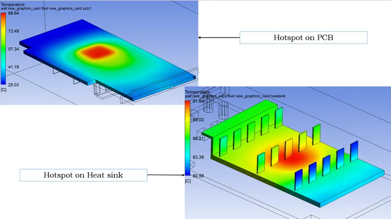
6) Hotspot in Assembly

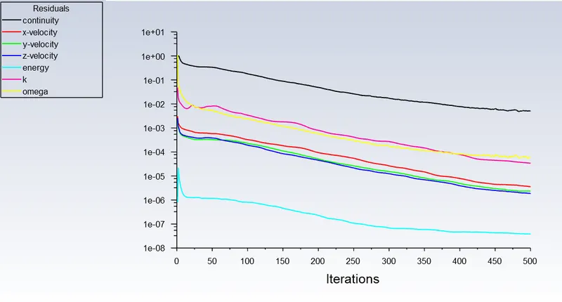
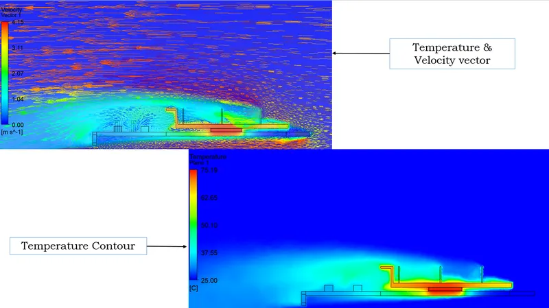
RESULTS: - CASE 6 (VELOCITY = 3.5 M/S)

1) Residual

2) Temperature graph

3) Heat transfer coefficient graph

4) Velocity vector and Temperature contour

5) Heat transfer coefficient contour

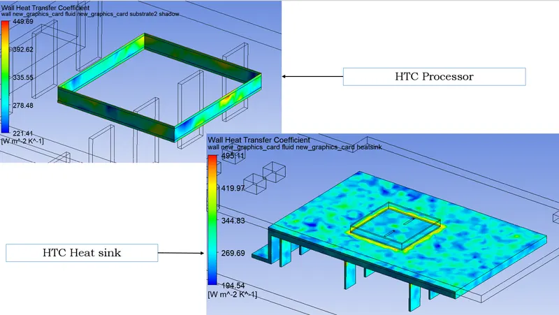
6) Hotspot in Assembly

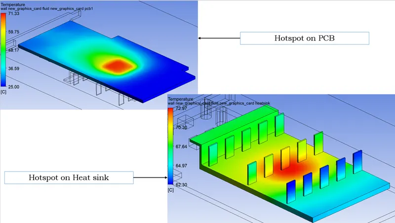
RESULTS: - CASE 7 (VELOCITY = 5 M/S)

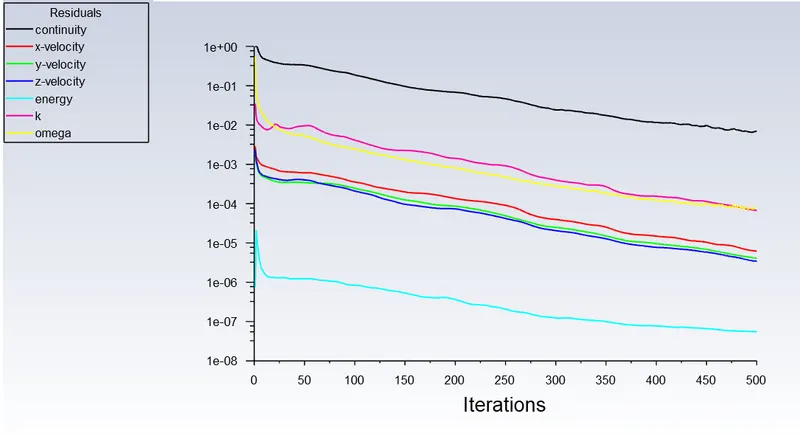
1) Residuels

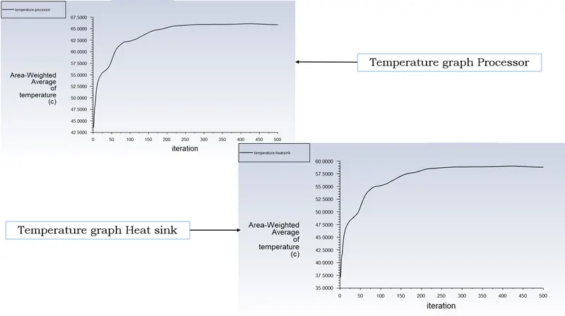
2) Temperature graph

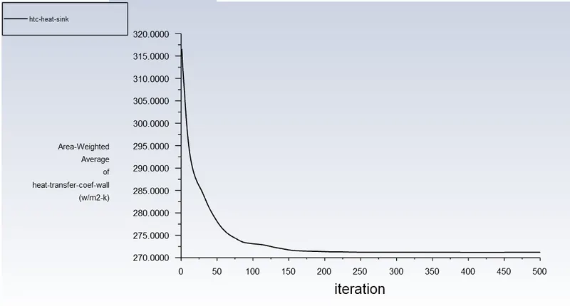
3) Heat transfer coefficient graph

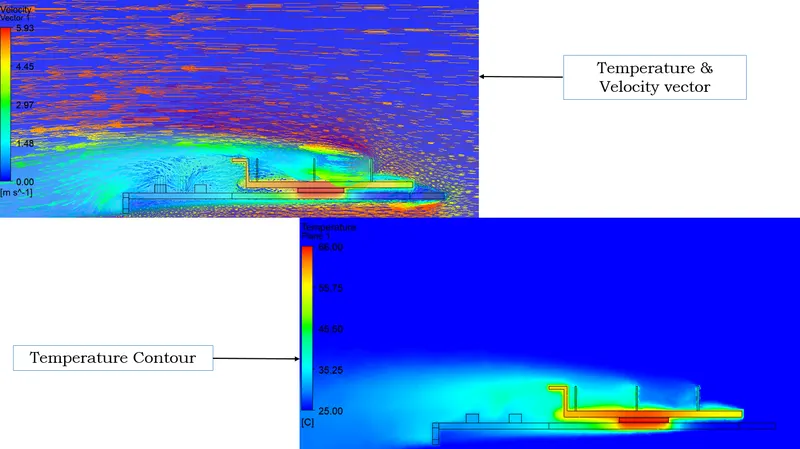
4) Velocity and Temperature contour

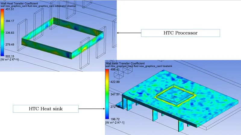
5) Heat transfer coefficient contour

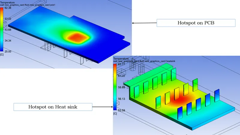
6) Hotspot in Assembly

RESULT TABLE

Parameters	Avg Temperature at Processor ℃	Avg Temperature at Heat sink ℃	Avg HTC on heat sink (W.m2/K)	Maximum Temperature at Heat sink ℃
Case 5 – Velocity 2m/s	93.90	86.73	266.84	91.84
Case 6 – Velocity 3.5 m/s	75.05	67.94	268.31	72.97
Case 7 – Velocity 5 m/s	65.86	58.78	271.21	63.77

Conclusion: -

• From the simulation of conjugate heat transfer of graphics card, the processor temperature is high enough going beyond the temperature limit of material if compared with real life temperature range.
• Mesh independent test is carried out and 0.25mm mesh size takes more time to simulate as compared with other mesh size simulation. So the mesh size which has been used for the rest of the simulation is 0.5mm minimum mesh size. This size provides the good accuracy of result with efficiency towards the computational time.
• The convergence of the results can be seen from the residual plot in which all the criteria related to flow field and energy equation are dropping with ease. If the number iteration is increase by another 200 then solution will be converged. Without relying on the residual plot for convergence of the solution, the plot like temperature graph on the processor and heat sink show that after 120 iterations it come steady state condition for all the simulations. The heat transfer coefficient in the mesh independent test is increased because the number of element for each cases has increased.
• Varying the velocity for same case setup show that temperature of the processor and heat sink is decreasing. The rate of heat transfer rate for each of the case has increased as velocity is increased. From the maximum temperature achieved by the processor is in the range for the 2m/s velocity is suitable for real life use of graphics card.