Week 6 - Multivariate Newton Rhapson Solver

Week 6 – Multivariate Newton Raphson Solver for Non-linear ODE

Aim: - Use of Multivariate Newton Raphson technique to solve system of stiff ODE system.

Objective: -

• To study the derivation of solving stiff ODE using implicit method.
• To derive the solution for stiff ODE using Multivariate Newton Raphson solver.
• To code the solution of stiff ODE using python.
• To plot the error for the problem.

Introduction: -

In view of solving differential equations with numerical integration methods, explicit and implicit approaches are mostly used to find the approximate solution of equations. When the differential equation has the variable which is input and output at the same time in function it gets difficult to construct the solution using implicit and explicit methods. The solution of equation of such stiff ODE can be done using Multivariate Newton Raphson method in which functions jacobian is used to solve the equation. Depending upon the type of numerical integration technique used the jacobian is used in both explicit and implicit.

The newton method is an iterative method to find the roots of differential function ‘F’. The multivariate newton method is improvement of single variable Newton-Raphson method. This is method mostly used for continuous systems which is differential with respect to multiple variables. To study the function let us assume that:

`f(x)=0`

where f is differentiable. It starts with the seed value of x¹ and recursively obtain the subsequent value of x², x³ and x⁴ and follows. At each of the value of x^k it need to construct a Jacobian approximation which is derivate of function with respect to x. It is given as:

`〖f'〗^k (x)=f(x^k )+Jf(x^k)(x-x^k)`

and if we select the x^k+1 as solution to

`f^'(k) (x)=0`

then:

`x^(k+1)=x^k- [J f(x^k )]^(-1) f(x)^k`

where J is the jacobian matrix which is basically a matric consisting the first order partial derivatives of multivariate system of equations

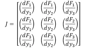
where

`F= [[F1],[F2],[F3]]`

In both the Newton methods there is issue with convergence. In Univariate method, if

`f^' (x^k )=0`

then that method is going to fail and convergence is never achieved. Similarly, if

`J f(x^k )=0`

is singular then Multivariate Newton Raphson method is also get failed at convergence. Issues of no solution or multiple solution can also be arise in this method.

Derivation for Equations: -

Given equation for finding out roots:

`1) (dy_1)/dt= -0.04y_1+(10)^4 y_2 y_3`

`2) (dy_2)/dt=0.04y_1-(10)^4 y_2 y_3-3 ∙(10)^7 y_2^2`

`3) (dy_3)/dt=3 ∙(10)^7 y_2^2`

Using the implicit scheme for creating the equation to find the value of y

`(y_1^n- y_1^((n-1) ))/(Δt)= -0.04y_1^n+(10)^4 y_2^n y_3^n`

`(y_2^n- y_2^((n-1) ))/(Δt)= -0.04y_1^n+(10)^4 y_2^n y_3^n-(3.10)^7 (y_2^n )^2`

`(y_3^n- y_3^((n-1) ))/(Δt)= 〖3.10〗^7 (y_2^n )^2`

for making more clear we will make some changes in equation which are given as:

`f_1= y_1^(n-1)+Δt (-0.04y_1^n+〖10〗^4 y_2^n y_3^n- y_1^n )=0`

`f_2= y_2^((n-1) )+Δt (-0.04y_1^n+〖10〗^4 y_2^n y_3^n-〖3.10〗^7 (y_2^n )^2 )- y_2^n=0`

`f_3= y_3^((n-1) )+Δt (〖3.10〗^7 (y_2^n )^2 )- y_3^n=0`

Using the matrix function for the above equation, the root finding using Multivariate Newton Raphson method is given by:

`Y_(New)=Y_(guess)-α (J^(-1) F)^n`

Coding Approach: -

The coding for the Multivariate Newton Raphson system goes same as it was done for implicit and explicit coding. The changes made in code under the definition of jacobian matrix and the loop of jacobian matrices. The code start with defining the function which are going to be used for getting solution of non-linear ODE. After that jacobian function is created to provide the first derivate of variable with respect to function.

Then initial conditions of problem are defined to find the roots of solution. It is important to create the old value roots to update for each of the iteration. After that time duration for solution is considered as 10 minutes and the time step of 0.1 is provided. From the both input the number of points are calculated which is ‘n’ and will be used for creation of loop. The dummy value of new root value is created so that it can be updated after each of the iterations also stored and used for plotting purpose. Then solver is imposed in the loop start from 0 to ‘n’. In solver function jacobian is used, also matrix multiplication is used to get new value of ‘y’. After the loop it is important to update the value of ‘y_old’ value with new ones. After updating the value, it required to create the error plot with respect to iteration which need to be decline so that error should be near to zero. After that in the code three subplots are created for showing convergence of each root value with respect to number of iterations.

The code is shown below:

"""
Solving ODE using Multivariate Newton Raphson Method
ODE equation are:
1) dy1/dt = -0.04y1 +10^4 y2y3
2) dy2/dt = 0.04y1 - 10^4 y2y3 - 3*10^7 y2^2
3) dy3/dt = 3*10^7 y2^2
Initial Conditions for Solution
y1 = 1, y2 = 0, y3 = 0
Code Written By: Shubham Chaudhari
Skill Lync - Week 6 Challenge
"""

import numpy as np
import numpy.linalg
import matplotlib.pyplot as plt

# Defining function for the solution


def f1(y1, y2, y3, y1_old, dt):
    return (y1_old + dt*(-0.04*y1 + 1e4*y2*y3)-y1)


def f2(y1, y2, y3, y2_old, dt):
    return (y2_old + dt*(0.04*y1-(1e4*y2*y3)- (3*1e7*y2*y2))-y2)


def f3(y1, y2, y3, y3_old, dt):
    return (y3_old + dt*(3e7*y2*y2)-y3)

# Creation of Function to Define Jacobian Matrix

def jacobian(y1, y2, y3, y1_old, y2_old, y3_old, dt):

    # Creation of 3 x 3 matrix
    j = np.ones((3, 3))

    # Defining step size for the solution
    h = 1e-6

    # Defining Row1 of Jacobian Matrix

    j[0,0] = (f1(y1+h, y2, y3, y1_old, dt)-f1(y1, y2, y3, y1_old, dt))/h
    j[0,1] = (f1(y1, y2+h, y3, y1_old, dt)-f1(y1, y2, y3, y1_old, dt))/h
    j[0,2] = (f1(y1, y2, y3+h, y1_old, dt)-f1(y1, y2, y3, y1_old, dt))/h

    # Defining Row2 of Jacobian Matrix
    j[1,0] = (f2(y1+h, y2, y3, y2_old, dt)-f2(y1, y2, y3, y2_old, dt))/h
    j[1,1] = (f2(y1, y2+h, y3, y2_old, dt)-f2(y1, y2, y3, y2_old, dt))/h
    j[1,2] = (f2(y1, y2, y3+h, y2_old, dt)-f2(y1, y2, y3, y2_old, dt))/h

    # Defining Row3 of Jacobian Matrix
    j[2,0] = (f3(y1+h, y2, y3, y3_old, dt)-f3(y1, y2, y3, y3_old, dt))/h
    j[2,1] = (f3(y1, y2+h, y3, y3_old, dt)-f3(y1, y2, y3, y3_old, dt))/h
    j[2,2] = (f3(y1, y2, y3+h, y3_old, dt)-f3(y1, y2, y3, y3_old, dt))/h

    return j

# Defining Initial Condition for Problem
y1_old = 1
y2_old = 0
y3_old = 0

# Creation of Matrix for old value of y
y_old = np.ones((3,1))
y_old[0] = y1_old
y_old[1] = y2_old
y_old[2] = y3_old

# Creation of Column Matrix for Function F
F = np.copy (y_old)

# Defining time step and solution time for problem
a = 1           # Under relaxation factor
t = 600         # Total time
dt = 0.1        # Time step size
n = int(t/dt)   # Number of solution points

# Creation of Array for storing updated value of y
y_new1 = []
y_new2 = []
y_new3 = []
it = []
error_up = []

# Considering iteration for solution
iter = 1

# Creation of Loop for calculation of roots of problem

for i in range(0, n):
    tol = 9e-6
    error = 9e9

    while error > tol:

        j = jacobian(y_old[0], y_old[1], y_old[2], y1_old, y2_old, y3_old, dt)

        # Function column vector matrix
        F[0] = f1(y_old[0], y_old[1], y_old[2], y1_old, dt);
        F[1] = f2(y_old[0], y_old[1], y_old[2], y2_old, dt);
        F[2] = f3(y_old[0], y_old[1], y_old[2], y3_old, dt);

        # Matrix Multiplication for solver

        y_new = y_old - a*np.matmul(numpy.linalg.inv(j),F);

        # Error estimation for solution convergence
        error = np.max(np.abs(y_new - y_old));
        print(error)

        # Updating the yold value
        y_old = y_new

    # Printing of Roots for problem

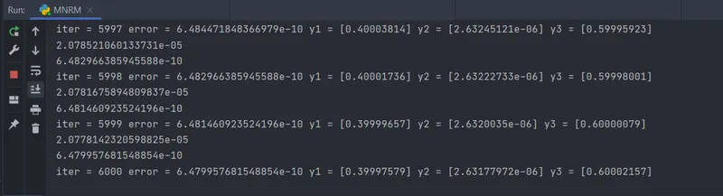
    log = 'iter = {0} error = {1} y1 = {2} y2 = {3} y3 = {4} '.format(iter, error, y_new[0], y_new[1], y_new[2])
    print(log)

    y_old = y_new
    y_new1.append(y_new[0])
    y_new2.append(y_new[1])
    y_new3.append(y_new[2])
    error_up.append(error)

    iter = iter+1
    it.append(iter)

    # Update of old value
    y1_old = y_new[0]
    y2_old = y_new[1]
    y3_old = y_new[2]

# Error plot
plt.plot(it,error_up,'--',color = 'red')
plt.yscale("log")
plt.title('Error Dropping Plot')
plt.xlabel('Number of Iterations')
plt.ylabel('Error Value')
plt.show()

# Figure creation for 3 row and 1 column
fig, ax = plt.subplots(3)
# Convergence of Y1 root value
ax[0].plot(it,y_new1)
ax[0].set_title('Convergence of Y1')
ax[0].grid('on')

# Convergence of Y2 root value
ax[1].semilogy(it,y_new2)
ax[1].set_title('Convergence of Y2')
ax[1].grid('on')

# Convergence of Y3 root value
ax[2].plot(it,y_new3)
ax[2].set_title('Convergence of Y3')
ax[2].grid('on')

fig.tight_layout()
plt.show()

Results

• Error plot

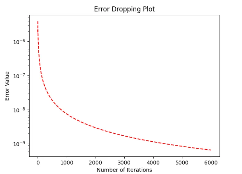
From the above it can be seen that the error is reducing for each of the iteration and lowers down giving information on the convergence has been reached and the value of roots are found accurately.

• Convergence Plot

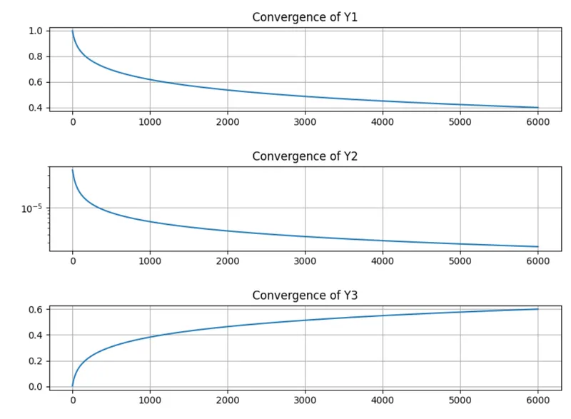
In above graph it can be see that each of the root value has near to convergence for a specific value. The value of Y1 = 0.3999, Y2 = 2.6317e-6, Y3 = 0.60002. If the step size is lowered again the graph will show straight line for this value which will be more assuring.