Week 1: Channel flow simulation using CONVERGE CFD
Week 1 – Challenge: - Channel Flow
Aim: - Performing a Channel flow test case in converge CFD software with different mesh settings.
Objectives: -
- To study the channel flow and its characteristics.
- To set up the case for the channel flow in the converge software.
- To use different mesh setting for the channel flow case and find the outputs.
- To run the simulation using parallel processor in Cygwin command prompt.
- To get velocity and pressure contours from paraview post-processor.
- To plot the velocity, mass flow rate, total pressure and cell count in converge software.
- To produce the animation of velocity profile in the paraview and give details of results obtained from simulations.
Introduction: -
Flows in the channel or conduits are have special science interest. Most of the time the channel flow is represent as the circular pipe flow or rectangular section flow. Similar to channel flow there is another term which represent open-channel flow which is most similar to channel flow theoretical region without boundaries at the end. The main aspect of study the channel flows are governed by the pressure differences. The flow under pipe are mostly cause due to the pressure different and are incompressible in nature. The another approach to study the channel flow is to determine the profile velocity inside the channel or tube. The rough boundary at the wall will create distorted velocity profile at the boundary which is part of study.
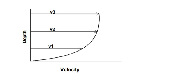
As it can be seen from above image the velocity gets decrease as it moves downward in depth. The parabolic nature of velocity profile is the validation of the channel flow test in this study. The velocity increases from zero at the invert of the channel to a maximum value close to water surface. The velocity difference results from the resistance of flow at the top and bottom layer of channel.
Solution Methodology: -
The Channel flow case set up is done with respect to pre-processing, solving and post-processing methodology. The Converge software offers user to create the geometry, generating the mesh and make the required solution setup. The geometry of the Channel flow is considered as 3D in nature but the solution is done on 2D base. The case is representing as plane stress problem where the stresses along Z axis are considered negligible. The channel flow is grid manipulation is done in three steps.
- Channel flow run 1 with 0.2mm mesh size.
- Channel flow run 2 with 0.15mm mesh size.
- Channel flow run 3 with 0.12mm mesh size.
For every mesh size the simulation was processed and results were compared with each other from paraview post-processor. The main function of converge software is to pre-processes the geometry, mesh and case setup. The solving of the problem is done from Cygwin which is a command prompt like window. The inputs files from the converge is need to be read from the Cygwin and it will solve the files just like OpenFoam software. Converge does not have sophisticated post-processor hence the output files are converted into readable files which paraview can understand.
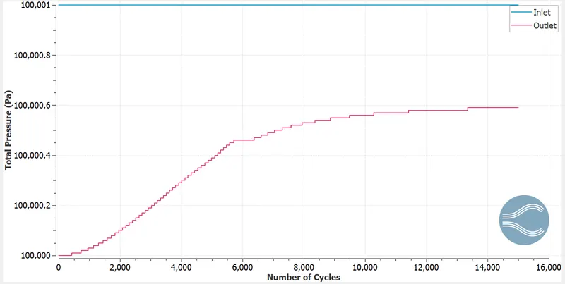
The flow inside the channel is considered as incompressible air with the species of O2 and N2 which are present in air. The steady state solver is used with PISO differential scheme. The flow is governed by the pressure difference caused at inlet and outlet. The initial pressure is kept constant which is equal to the inlet pressure.
Geometry: -
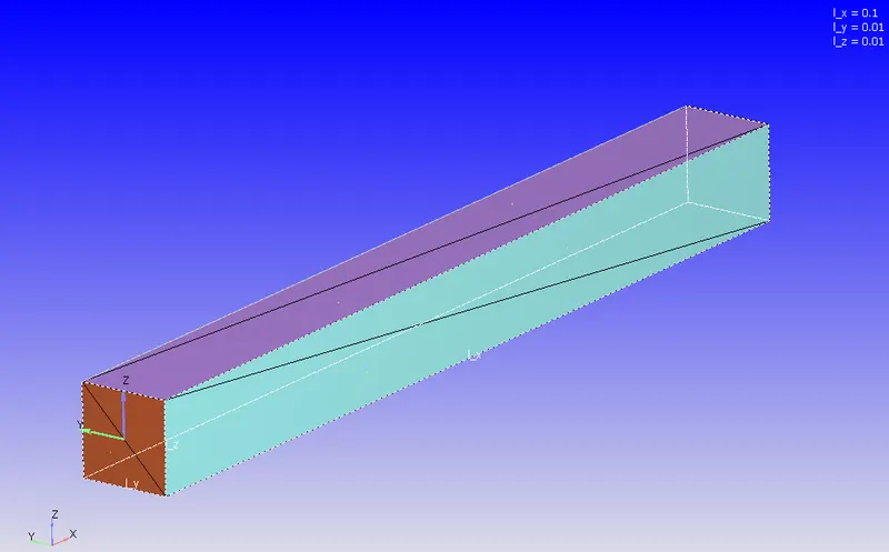
The geometry is 3D in space was created in the converge studio. The dimension of geometry is 0.1m in X axis, 1e-2 in Y and Z axis respectively. This geometry is created from the geometry tab in converge where the box type of geometry is selected and the dimension was provided accordingly. After creating the geometry, it has been stich with boundary which is most important part in the simulation. The geometry is representing as bunch of triangles in the viewport of converge software. They have been bind as boundary to act as a surface of the box. This is done by boundary option in the geometry subtabs. For the simulation inlet, outlet, top-bottom face, front and back 2d wall boundaries are created. It is important to set the normal of the face in the right direction to make the flow happen inside the Channel. After completing this steps the final geometry is shown below:
Case Setup: -
The case setup has been started with selecting the application type of the simulation which is time based initially. As the Converge 3.0 software did not allow permission to directly set the steady state simulation compared with earlier versions. The steady state approach has to be selected in later case setup settings. The material for the simulation is been considered as Air with species interaction. As the Converge is mostly used for combustion simulation hence the material should have species involvement or else it will throw an error as no species in the mech.dat file which eventually result in no simulation process.
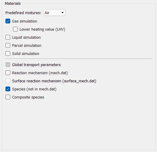
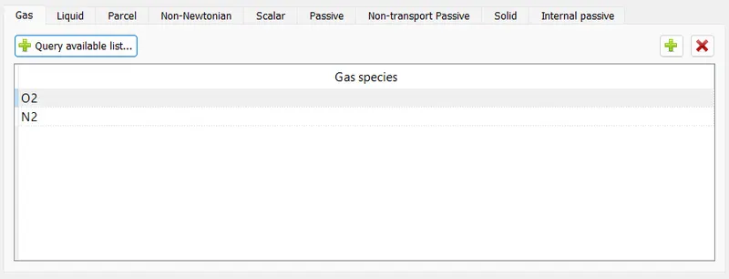
In material tab case setup other properties like Equation of state, critical temperature and pressure are assigned automatically. The global transport properties have to be kept default for simulation. The species are necessary to define in the simulation. The air contains oxygen and nitrogen and has to be incorporated.
After completing the material selection, simulation parameters need to be defined. In which first and foremost important is the what type of solver is used for the simulation. In this case the steady state solver with full hydrodynamic mode and compressible gas flow solver has been used. In the miscellaneous tab momentum, species and steady state monitor has to be checked for the simulation.
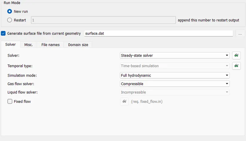
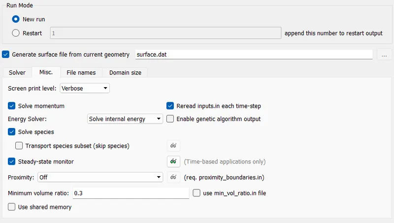
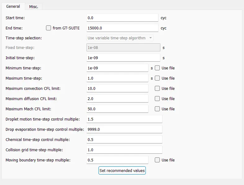
The solution has been run for 15000 cycles. Converge software offers user to go with number of cycles or with the time period. As it is a steady state simulation going with the number of cycles is better practice.
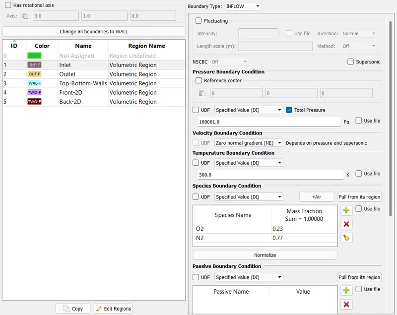
As it was earlier mentioned that, the geometry has boundary defined. This boundary is used as the flow governing boundary conditions like inlet, outlet, walls and 2D walls. Converge provide good color representation to these boundaries for better view and selection. User can manipulate the color depending upon ease of selection. The inlet is set as ‘INFlOW’ boundary condition in which pressure of 100001.0 Pascal’s is defined. The velocity boundary conditions are defined as zero normal gradient. The air that is coming from inlet has to be defined in species form with mass fraction of total 1.
Similar to inlet, outlet boundary condition is defined as ‘OUTFLOW’ In which outlet pressure is set to be as 100000.0 Pascal’s. As the air defined in the inlet similar to it outlet has to be defined with species fraction of air.
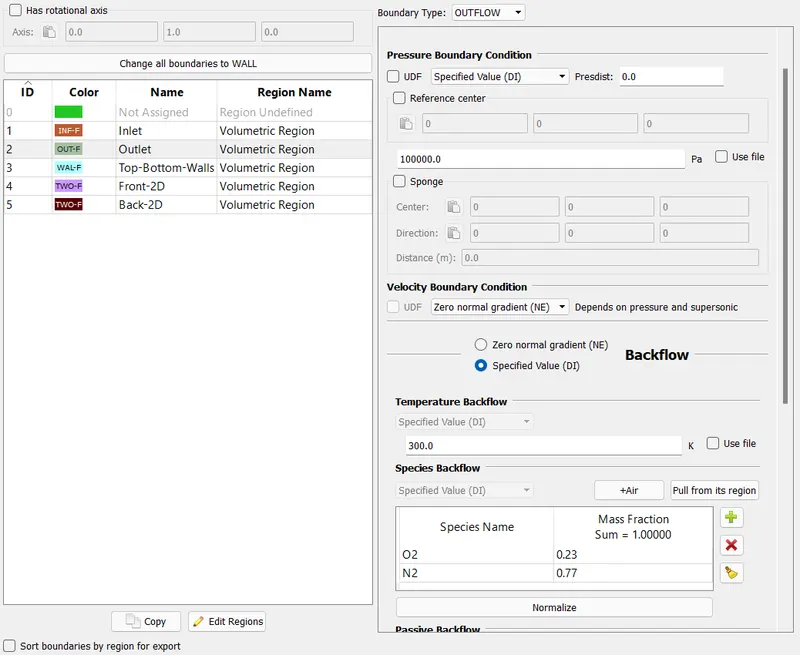
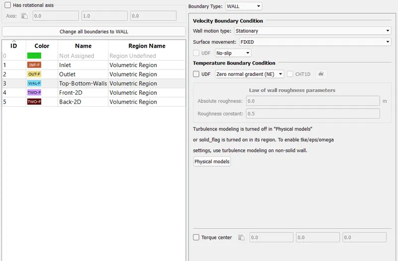
The top and bottom surfaces are treated as walls and front face and back face are treated as 2D walls. It is important to represent the front and back face as 2D as the simulation is happened in space in which Z direction is considered as infinite in length. The walls are treated as no-slip boundary condition as no roughness at the top and bottom are considered.
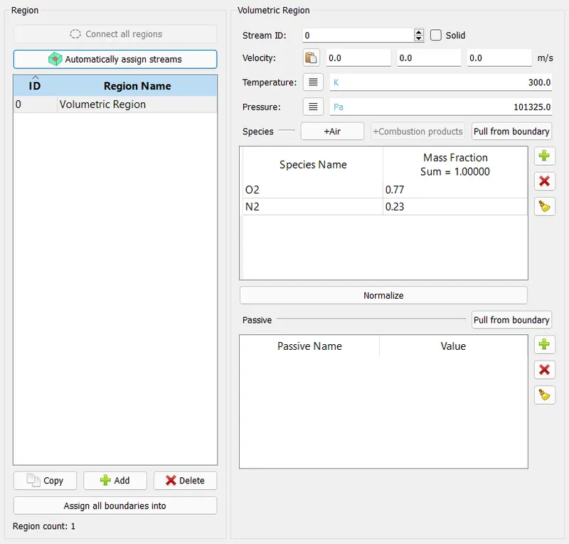
The partial differential equation of the Navier stokes equation in the fluid domain are solved in small discrete volume. Hence it is important to create the 3D domain in which this governing equation need to be solved. In converge this can be created by assembling the region of surface and provide the initial conditions to it. This can be done in Region and Initialization tab in the case setup. In this section initial pressure and temperature with species has to be define and this region then assigned to the boundary so that it can be read by solver.
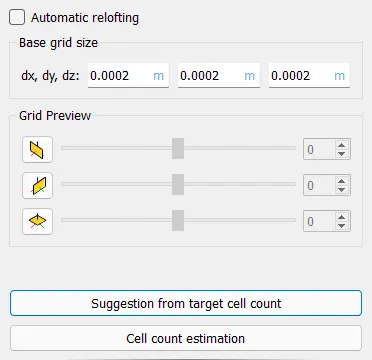
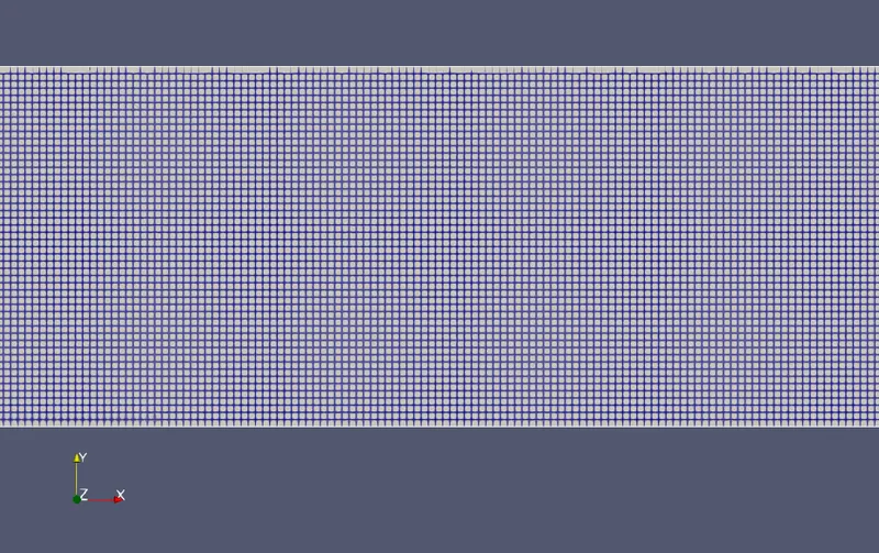
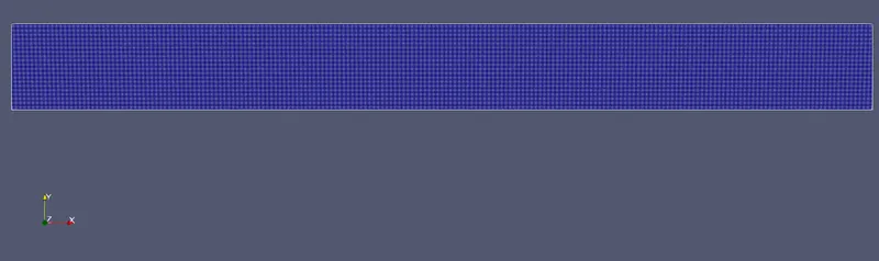
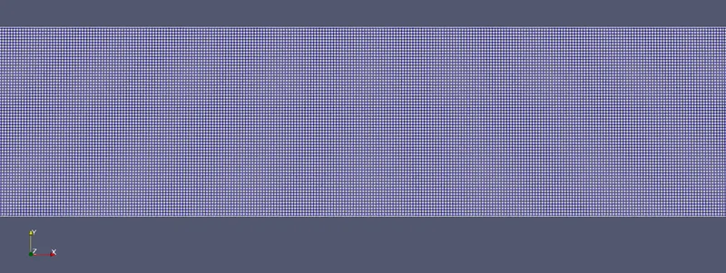
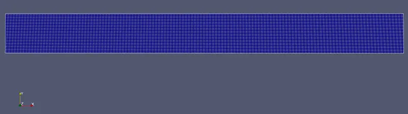
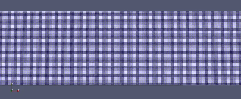
After completion of region defining, the base grid has to be selected. For the first case the overall mesh size in x, y and z direction is taken as 2e-4 in meters. It is need to note that the cell count of mesh size should not go beyond 5 million cells or it will result in no simulation.
For plotting the results in the Converge itself, the post output variable has to be selected for solution process. For the steady state simulation variables like velocity, pressure, mass flow rate, temperature and density are selected. Similar flow variables, geometry variables like region ID is selected. It is important to select the species in the mass fraction of output variable as they were need to be solve along with fluid flow governing equations. This can be done in same window in which species and passive value are defined.
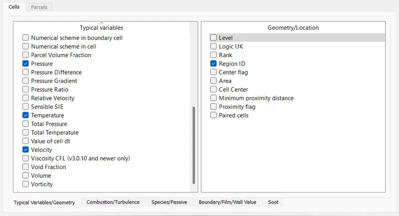
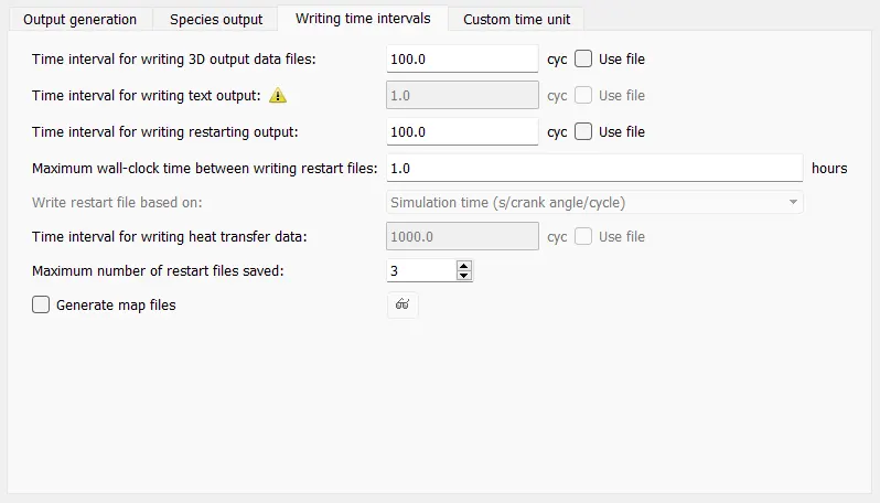
The simulation has been set up for 15000 cycles. It is necessary to select the time period for which the output files have to be written. This output files can be used to create the contour, time plots and animation. Along with output files, the restart files have to be generated with simulation. This restart files can be used when the simulation can be interrupted due to sudden crash of system.
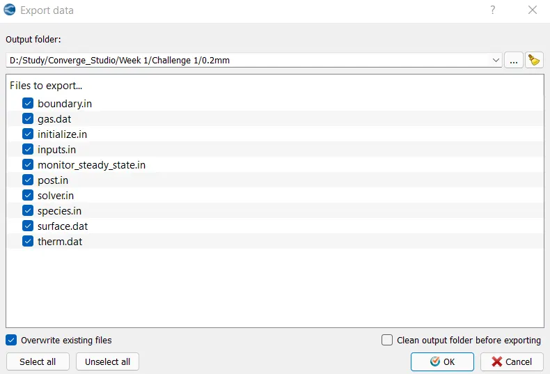
After completing the whole case set up process. This set up files has to be exported into a certain folder where converge solver executable is available. This files have to be called by Cygwin command prompt and need to be run accordingly in parallel or in serial processor. The files are shown below:
Results: -
Case 1- Mesh Size (dx=dy=dz = 2e-4 m)
- Mesh Size
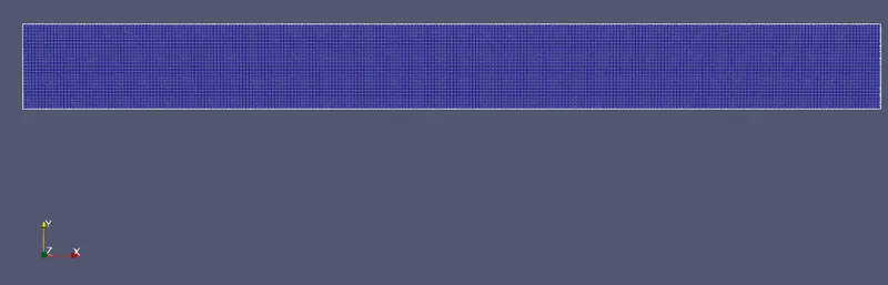
- Expand View of Mesh
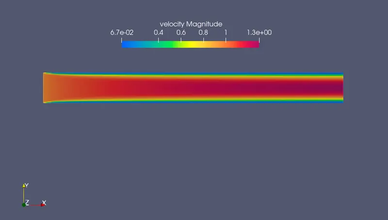
- Velocity Contour
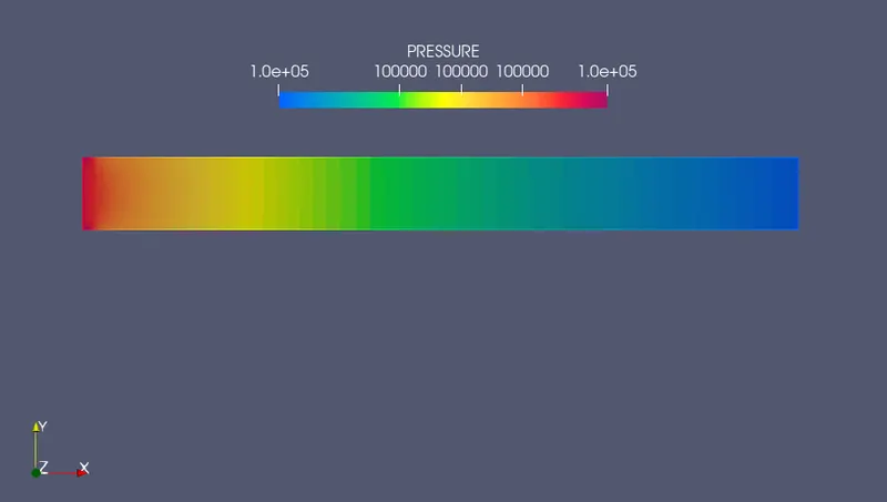
- Pressure Contour
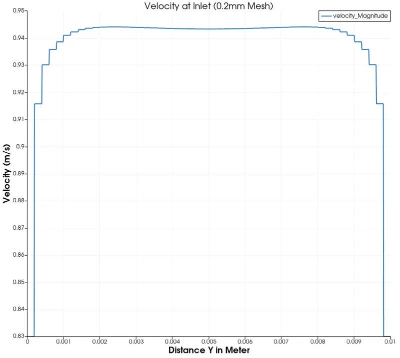
- Velocity Plot at Inlet
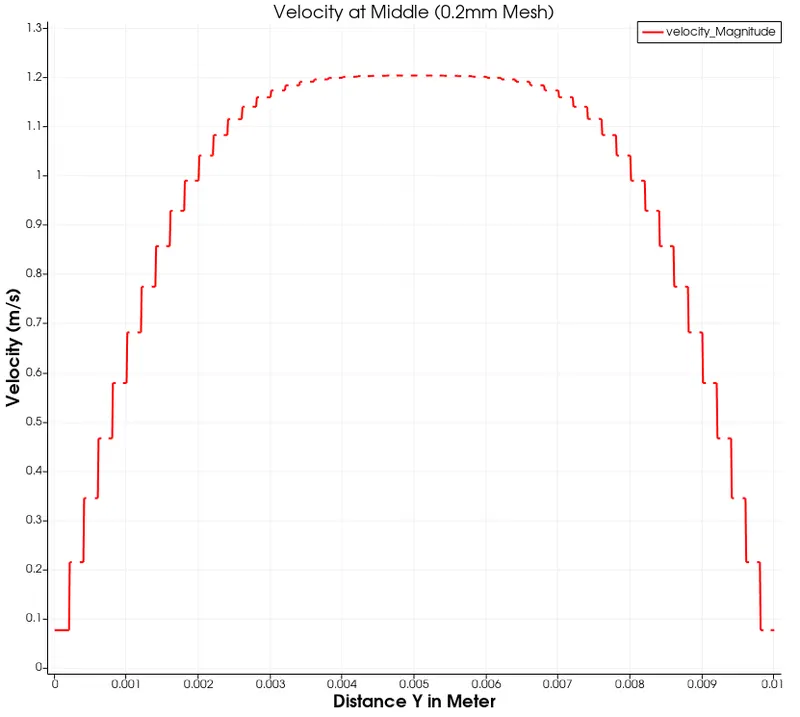
- Velocity Plot at 0.05 m In X axis
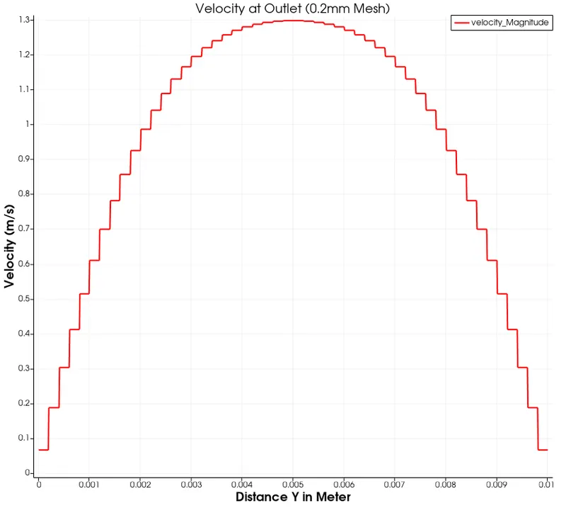
- Velocity at Outlet
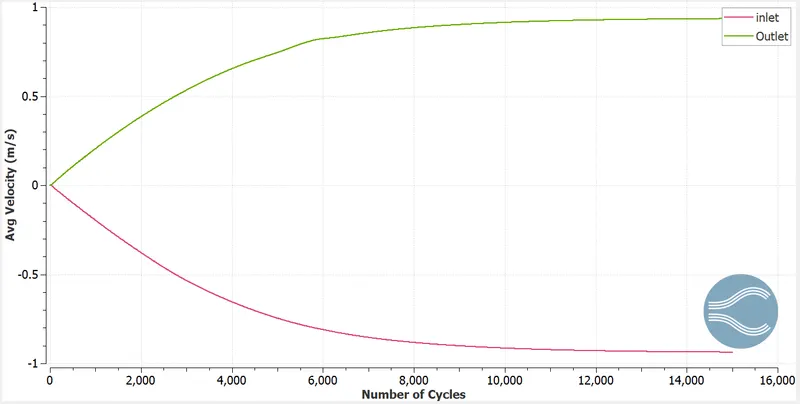
- Average Velocity Graph at Inlet & Outlet
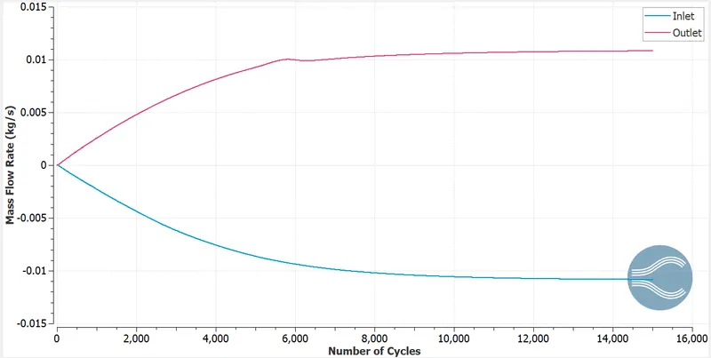
- Mass flow rate Graph at Inlet & Outlet
- Total Pressure Graph at Inlet & Outlet
- Total Cells Graph
- Animation YouTube Video Link
Case 2- Mesh Size (dx=dy=dz = 1.5e-4 m)
- Mesh Size
- Expanded View of Mesh
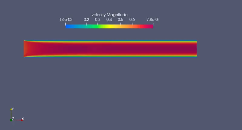
- Velocity Contour
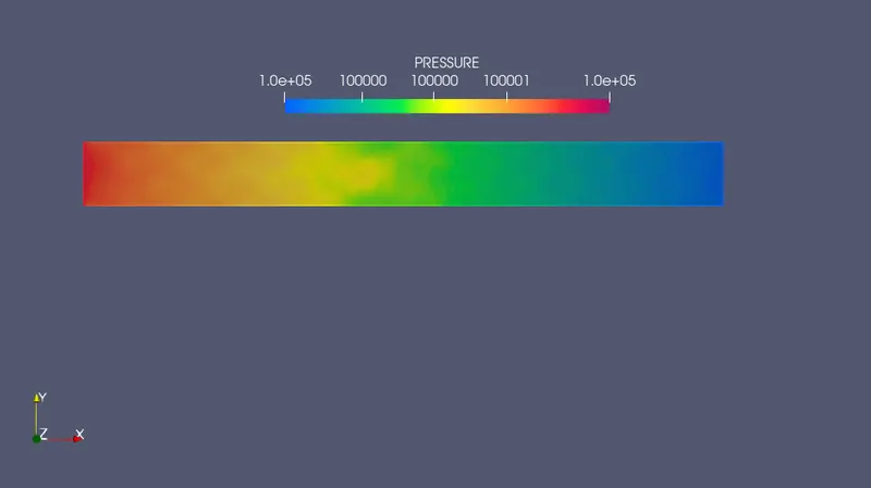
- Pressure Contour
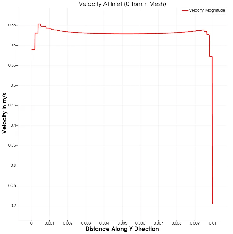
- Velocity Plot at Inlet
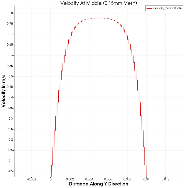
- Velocity Plot at 0.05 m in X axis
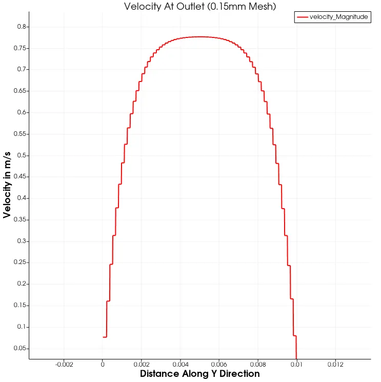
- Velocity Plot at Outlet
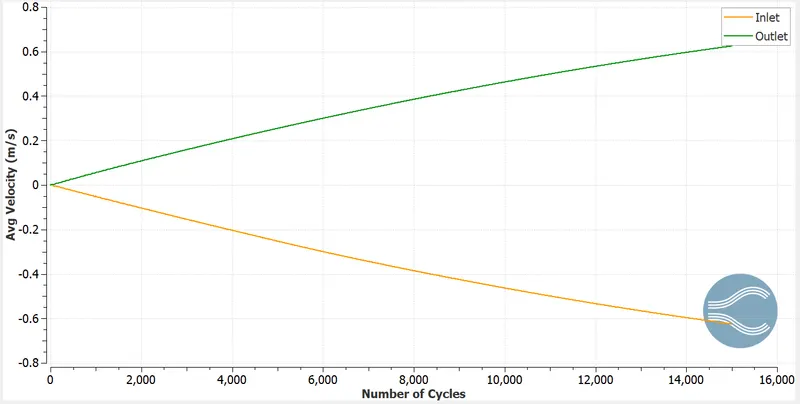
- Average Velocity Graph at Inlet & Outlet
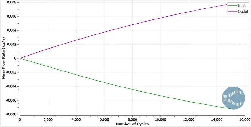
- Mass flow rate at Inlet & Outlet
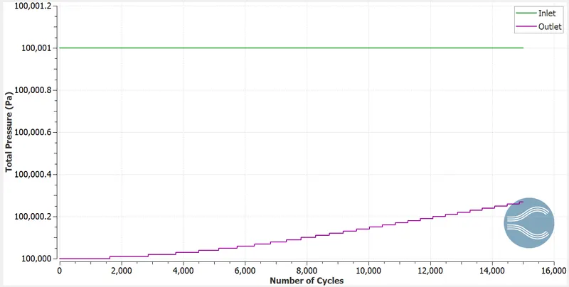
- Total Pressure Graph at Inlet & Outlet
- Total Cell Count Graph
- Animation YouTube Video Link
Case 3- Mesh Size (dx=dy=dz = 1.2e-4 m)
- Mesh Size
- Expanded View of Mesh
- Velocity Contour
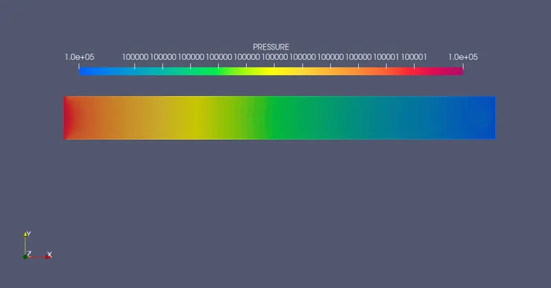
- Pressure Contour
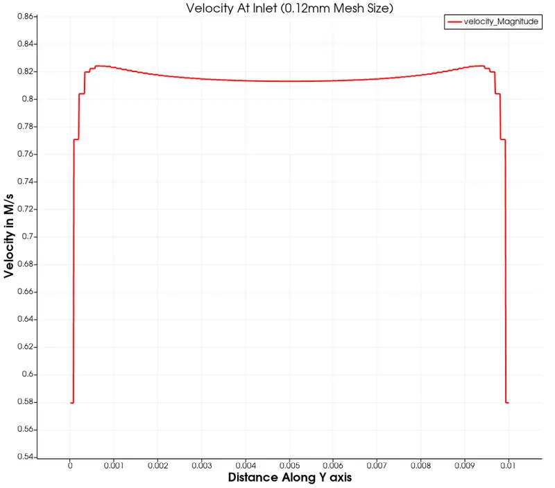
- Velocity Plot at Inlet
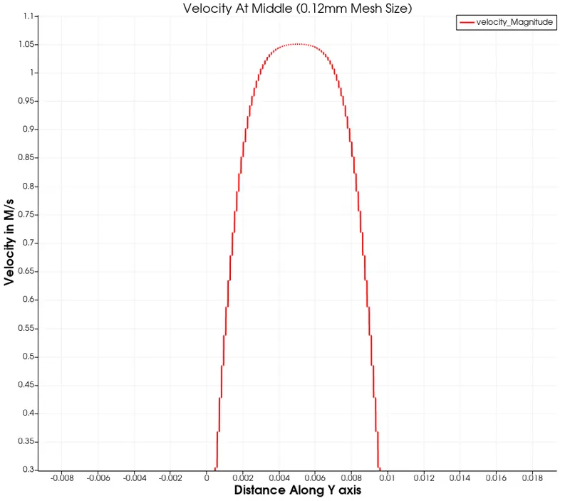
- Velocity Plot at 0.05 M in X Axis
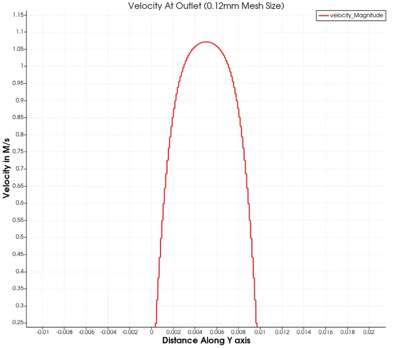
- Velocity at Outlet
- Average Velocity Graph at Inlet & Outlet
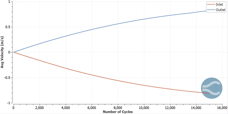
- Mass Flow Rate Graph at Inlet & Outlet
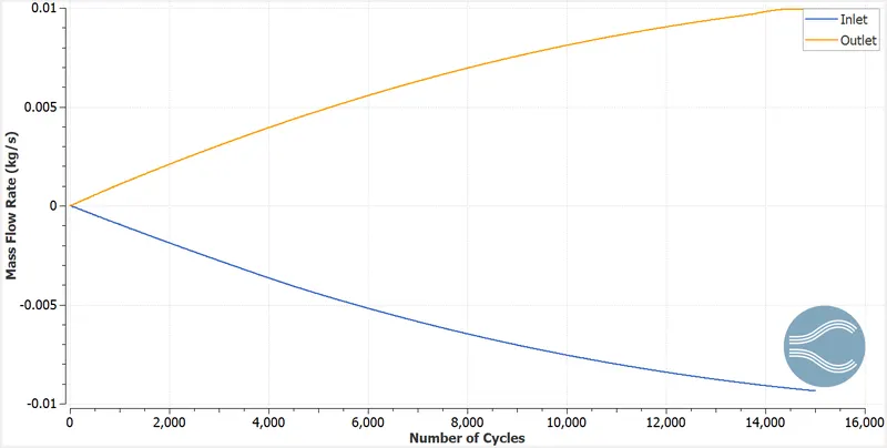
- Total Pressure Graph at Inlet & Outlet
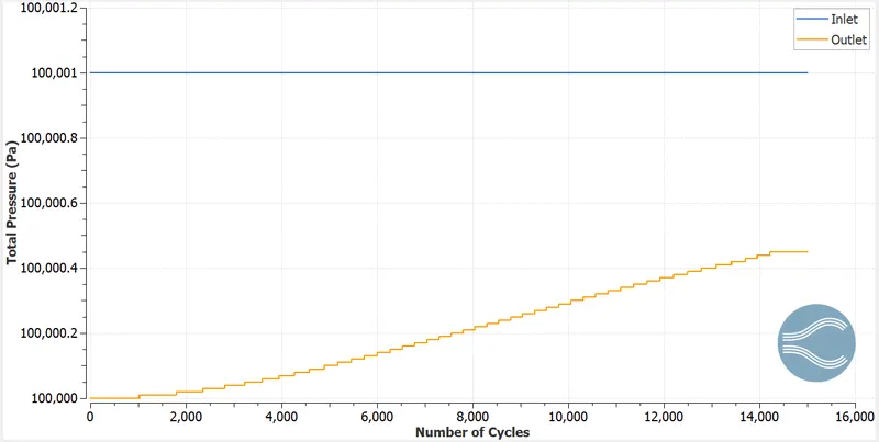
- Total Cell Count Graph
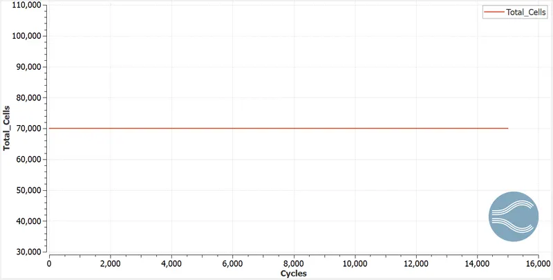
- Animation YouTube Video Link
Observations: -
1) From the observation of contour it can be seen that the flow is governed with pressure difference.
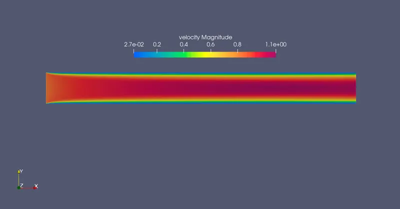
2) From the velocity contour plot, at the inlet the velocity profile is mostly straight line and at the middle of the domain the velocity profile looks parabolic but the highest velocity value has not been reached. In the velocity plot at outlet it can seen that whole parabolic profile with highest velocity value.
3) From the velocity contour and the velocity plot, velocity at the top and bottom wall is near to zero and at the center is maximum. This cause by the no slip boundary condition at the walls.
4) From the graph of average velocity and mass flow rate for inlet and outlet both look same but the inverse in nature. This show the simulation obeys laws of mass conservation.
5) From the pressure graph for all the three cases it seems that pressure at inlet is constant but the pressure at the outlet is trying to attained equilibrium but at the convergence it is less as compare to inlet. This is the reason why the flow inside the channel is creating.
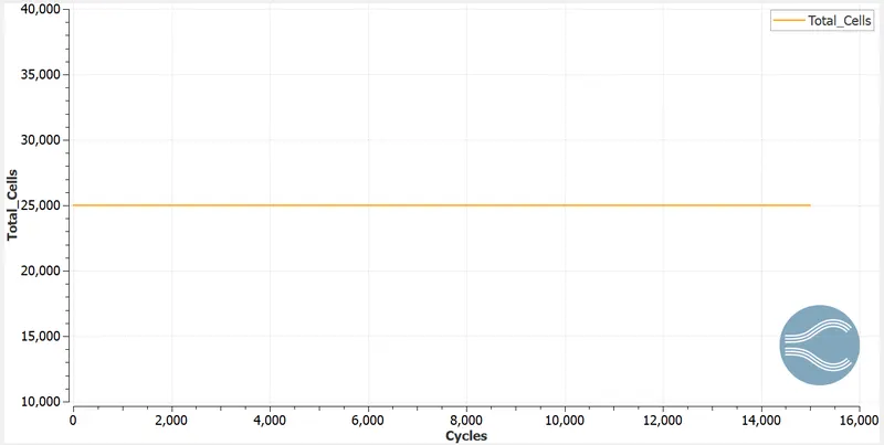
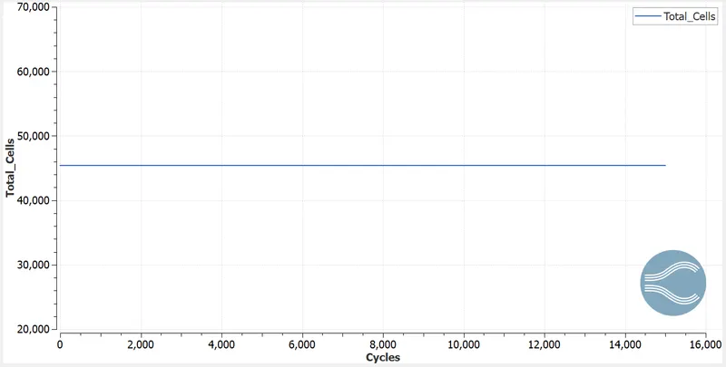
6) From the cell count graph it can be seen that, for each case the number of cell count is constant and as the mesh size is increasing the number of cell count is increasing for each case. Increase in number of cell cause the simulation to take more time for solving.
7) From the animation of velocity contour, it can be seen that the initially the velocity is constant throughout the domain. After some cycles the profile in the domain started creating. In the end it can be seen that no-slip region and velocity with high flow region created.
Link of Project
https://skill-lync.com/student-projects/channel-flow-simulation-using-converge-studio-3-0-software