Week 3 - External flow simulation over an Ahmed body.

Aim: - Validation of External air flow over Ahmed Body.

Objectives: -

• To study the Ahmed body as basic of simulation for external flow over vehicle.
• To study the evaluation of Y+ value and its importance for simulation.
• To pre-process the geometry and mesh for Ahmed body simulation.
• To refine the mesh and study the effect of coefficient of drag on the Ahmed body.
• To perform the mesh independent test for Ahmed body simulation.

Introduction: -

Turbulence is one of the phenomenon which need to be studied for development of car body and other features of car utility. The wake region behind the vehicle are very important to determine the slope behind the car. Ahmed body is a structure is mostly used to study the turbulence created by flowing air. Varying the slope of Ahmed body is used the study the vortices created behind the body. Flow separation and negative pressure development are main aspect studied accordingly. To study the actual car in wind tunnel test is complex due to its body design and employment of measuring accessories in wind tunnel, hence to study the drag force and respective coefficient, most of researcher has created the dimension of car which can be studied as the replacement of actual one which called Ahmed body. In most of the simulation the slant angle is changed to study the flow separation over the body. There are many literature has been provided in which both numerical simulation and experimentation has been carried out for the validation.

Flow separation has more importance in study of fluid dynamic as it will create more emphasis in measurement of pressure. The velocity which has been used for simulating the flow around Ahmed body is around 3 to 55m/s. To capture the flow around the Ahmed body it is important to have finer mesh region around the edges. To have better mesh resolution calculation of Y+ value become essential to capture the flow near body. Calculation of Y+ value is depending upon free stream velocity and skin friction coefficient of body.

In this simulation similar work has been carried out for flow around the Ahmed body. Simulation consist of free stream velocity of 25m/s and no slip conditions are applied to the surface. The main objective of this simulation is to find generation of vortices in the wake region of body. Another objective is to determine the Reynolds number and calculation of Y+ value for the simulation. Reynolds number calculation is depending upon dynamic viscosity of fluid, velocity of fluid, density of fluid and length over which flow is happening. In the case of Ahmed body simulation, the total length of body is considered as the length parameter for the calculation of Reynolds number. The Reynolds number is given by:

`Re=(ρVL)/μ`

Where,

Re = Reynolds number

ρ = Density of Fluid

V = Velocity of Fluid

L = Characteristic length.

µ = Dynamic viscosity.

The dimension of Ahmed body for this simulation is given below:

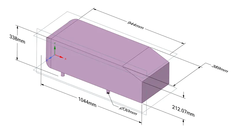
As we can see the total length of Ahmed body is 1044 mm and width is 389 mm with total height is 338 mm. The slant angle for which simulation is performed is 20°. The Reynolds number calculated for Ahmed body is given as:

`Re=(ρVL)/μ=(1.225*25*1.044)/(1.789e^(-5) ) =1786772.10`

The Reynolds number calculated is beyond laminar region hence it is important to add turbulence model for simulation. Use of correct turbulence model is depending upon treatment to boundary layer theory. Boundary layer theory suggest that the skin friction coefficient or shear stress is increase as flow past the body and create vortices in further down to the length of body. This area is seeming to be seen as the point of separation of flow. To capture point of separation and treat the problem with correct boundary layer phenomenon it is important to provide required Y plus value to the domain where fluid flow can be perfectly simulated in the vicinity of turbulence.

The desired first layer thickness of Y plus value is determine by calculating skin friction coefficient which is given as:

`C_f=0.026/(Re^(1/7) )`

After that wall shear stress can be calculated which is given as:

`τ_(wall)=(C_f*ρ*U^2)/2`

From calculation of shear stress near wall we can find frictional velocity which is given as:

`U_(Fric)= √(τ_(wall)/ρ)`

To calculate the first layer thickness it is important to decide the desired Y+ value for the calculation, depending upon the turbulence layer theory or wall treatment method the requirement of Y+ value is varied accordingly. The first layer thickness is given as:

`ΔS=(Y^+*μ)/(U_(Fric)*ρ)`

Solving & Modelling Approach: -

The flow over Ahmed body is external which means we required only outer shape of body to simulate the flow. For an external flow simulation, the fluid volume should present outside the experimented body. This can be overcome by the modeling software of ANSYS using space-claim. The modelling approach start with making volume outside the body and then removing the body so that only shape will present rather than body.

The simulation will be done in five stages in first one we will perform only baseline simulation to have understanding of mesh and solver setup. In second stage we will perform simulation by introducing another fluid volume inside original one with same mesh size and calculate the results respectively. We will check the plot of drag coefficient and lift coefficient as simulation progresses. In third state we will lower mesh size and provide inflation after calculating Y plus value for required case. In forth case we will again lower the mesh size and trying to figure out which mesh size is required for simulation as mesh independent test. In the last case we will again lower the mesh size and see how the result varying with respect to given drag coefficient value.

Case 1 - Flow simulation with default mesh setup.

Case 2 – Flow simulation with 0.1m mesh size for all bodies.

Case 3 – Flow simulation with 0.1m for outside enclosure and 0.05m for inside enclosure with inflation layers.

Case 4 – Flow simulation with 0.05m mesh size for outside enclosure and 0.025m mesh size for inside enclosure with inflation layer.

Case 5 – Flow simulation with 0.05m mesh size for outside enclosure and 0.010m for inside enclosure with inflation layers.

The flow parameter is default as of FLUENT provided. The fluid which is used for simulation is air and the velocity with which it travels across the domain is 25m/s. Pressure outside is atmospheric. There is no need to provide the energy equation as we are not interested in calculating temperature around the body. The solver which will be used for simulation is pressure based neglecting fluid compressibility effects. It is important to treat the problem by using Mach number which can be determine from flow velocity or Reynolds number. For most of problem where compressibility effects are taken into consideration meaning change of density during flow, density based solver are used in which implicit and explicit pressure-velocity coupling methods are used. For normal solver where density is not function of time and space, pressure based solver are used in which different methods are used as interpolation schemes.

Another modelling approach which we can use in this simulation is conformal mesh. Conformal and non-conformal mesh are very distinctive and have their own advantage and disadvantages. Conformal mesh is the mesh where mesh point is connected irrespective of different volume come together whereas non-conformal mesh is where mesh points are not connected respective of number of volume present in the simulation. The data reading in conformal mesh are easy and mostly accepted in fluid flow simulation. In non-conformal mesh, mesh interface is act as the boundary value which are used to calculate governing equation in next region. It is important to have practice of creating conformal mesh in CFD as it mostly acknowledge throughout the domain.

Pre-Processing- Geometry: -

To have accurate simulation at the end it is necessary to devote more time in pre-processing and meshing which makes life easier. For this simulation as discuss for the first state we will create a normal mesh of whole domain and then try to simulate it to know the solver setup and results respectively. The pre-processing start with importing the geometry of Ahmed body into pre-processor called Space-claim. After importing the geometry, it is very well known that we are simulating external flow simulation hence does require an outer fluid domain. This can be done by the tool called enclosure in Space-claim. What enclosure does is, it will create and domain as per used required with some dimension which act as fluid. After creating that enclosure, it is required to remove the body on which external flow simulation has to be carried out if we are not interested in the flow inside the body. After creating first enclosure, the setup will look like:

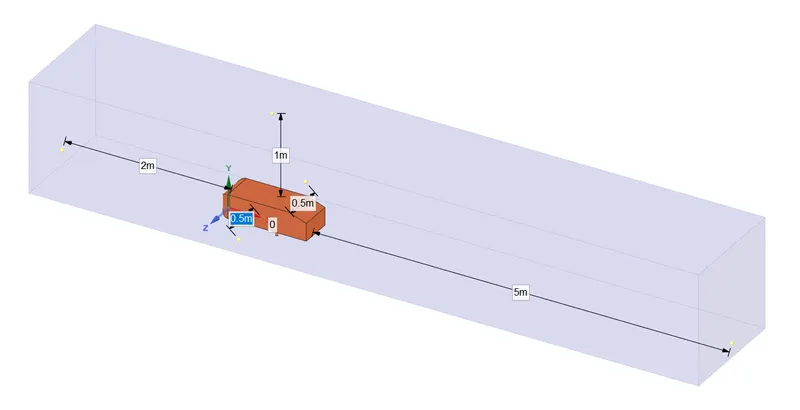
we can observe from above figure that; we have not selected symmetric dimension for the body as we would not get any freedom to give user defined value. The enclosure starts with basic dimension of 0.26m and then in each direction we can provide value. The inlet will be from 2m ahead of body and outlet will be 5m from the body. The side distance from the body are 0.5m and bottom is zero. Making the domain bigger will create further computation effort for solving the problem, hence it is importance to start with baseline simulation in which each factor is considered before making it to solver setup. The geometry after inserting first enclosure will look like

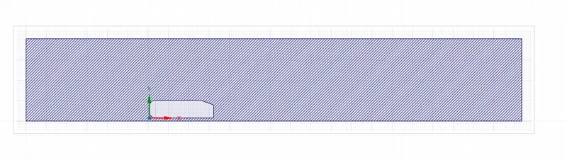
After completing first enclosure it is important to have another enclosure to have better mesh resolution near the body. If we are meshing first enclosure with lower element size it will create huge number of element in the domain which makes life difficult for simulation. Hence it is important have another region inside first one to have better mesh control near the Ahmed body. This can be seen as below:

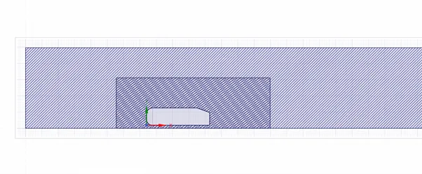
from above figure we can see that both the enclosure is overlapping each other which is not acceptable for simulation. This can be overcome by using interference option in space-claim. After applying the tool, the final geometry will be look like:

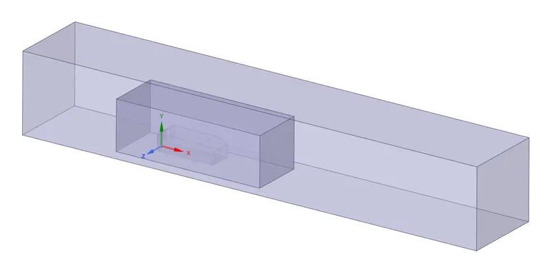
Pre-Processing- Meshing (Case 1): -

After completing geometry cleanup for simulation another stage is to mesh the geometry with correct mesh size for having converged results. For case 1 we are using only some features of global mesh control to get final mesh. The global mesh control provides mesh size to each of geometry present in the workbench. For case 1 simulation we are just using the default option of mesh generation to get mesh. Also we not interested in to provide inflation layer to Ahmed body. After completing mesh operation, the setup will look like:

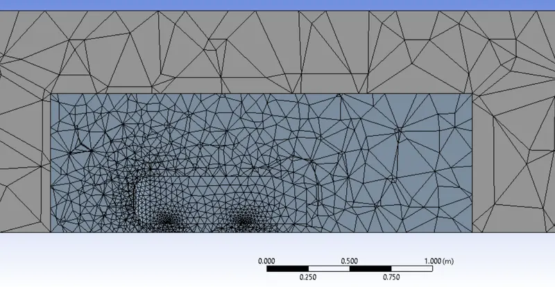
The amount of element created in baseline mesh are 80455. As we can see from the image above the finer size mesh element are created near the geometry where defeaturing is more. We are solving whole setup of Ahmed body as rather than half model because of availability high computational power.

Pre-processing – Solver Setup: -

For the solver setup as discussed earlier, we have used pressure based solver rather than density based solver by calculating Reynolds number for flow. The fluid which is used throughout the simulation is air and the properties are given below:

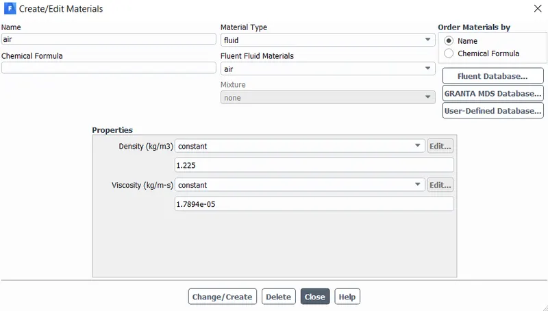
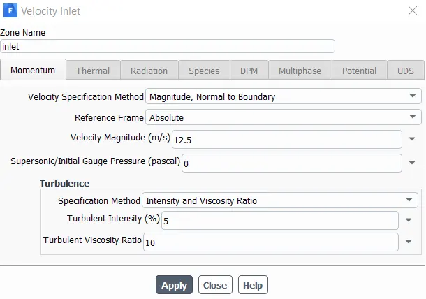
The next and most important thing in the simulation is boundary conditions. The inlet boundary condition is considered as velocity inlet of 25m/s and outlet boundary condition is treated as pressure outlet and considered as atmospheric pressure. It is necessary to define the car-wall as boundary of wall with no-slip conditions to evaluate drag and lift coefficients. The velocity inlet value is given as:

The turbulence model which is used for the simulation is k-epsilon with standard model having standard wall function as near wall treatment. This model provides great result accuracy near the wall of Ahmed body. The calculation of Y plus value is also depend on the which wall treatment is used.

For the calculation of lift and drag coefficient reference value are main attribute need to be provided in the simulation. Depending upon the area and length specification also from what boundary condition this value are calculated is required. As FLUENT does not have clue from which area this value has to be calculated. The frontal area of the Ahmed body is 0.185m² and length is 1.044m. This value has been provided in the reference value.

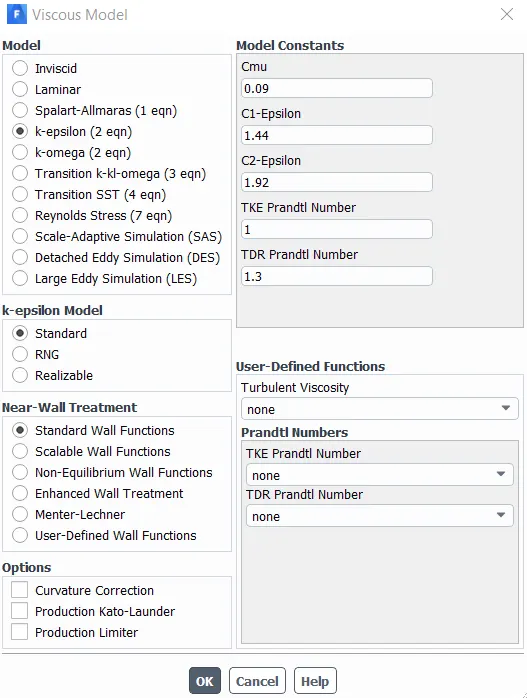
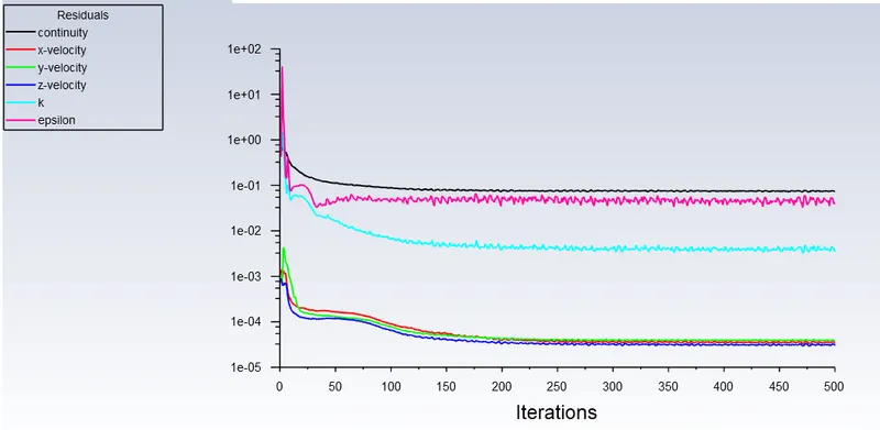
After providing every value for simulation the last setup is to choose the pressure-velocity coupling scheme for problem. The SIMPLE algorithm has been choosing for the problem with default settings. Before making initialization to the problem the reports need to be generated which are drag coefficient and lift coefficient. This can be accessed from solution report option in FLUENT. In solution report option forces has to be select which further provide option to select drag and lift coefficient or forces. It is necessary to select the wall on which this coefficient has to be calculated. After this it is important to see the solution animation as it progresses throughout the simulation process. For solution animation it required the reference frame or plane on which it will show the results. This can be done by using location option in which user can create plane, surface or point to be used as reference for solution. After making reference plane, to create solution animation initialization of problem has to be done before. The number of iteration are around 500 in which each of the value will be calculated.

Post-Processing (Case 1 – Default Mesh Setup): -

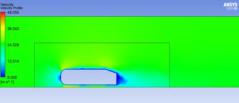
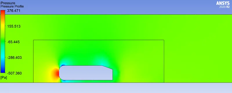
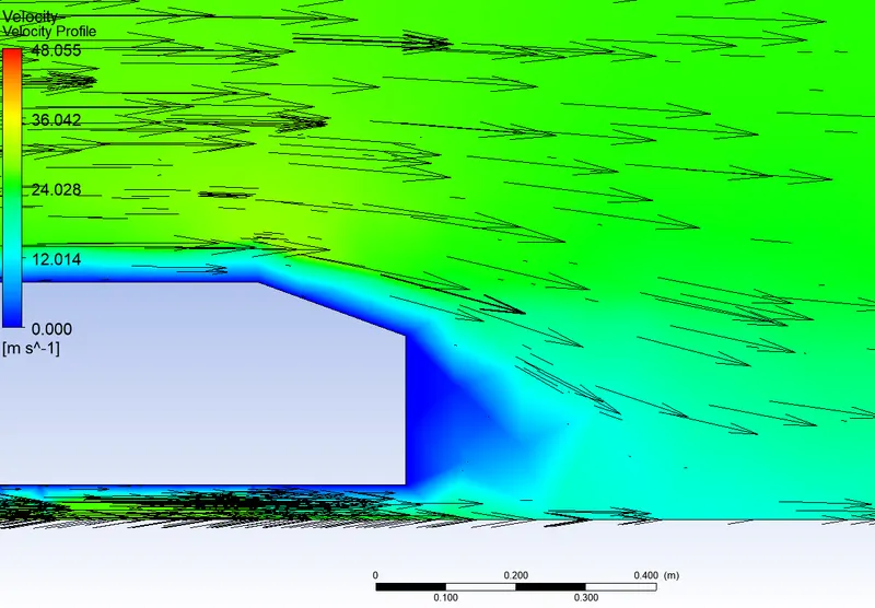
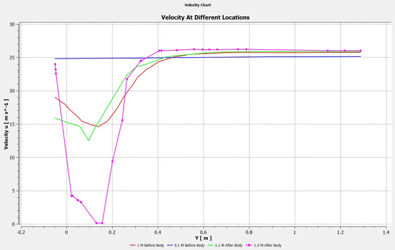
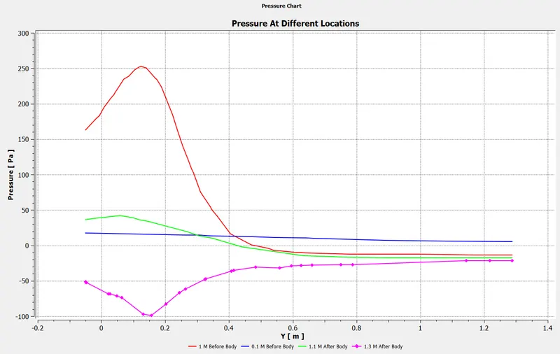
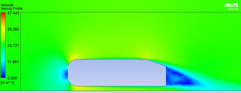
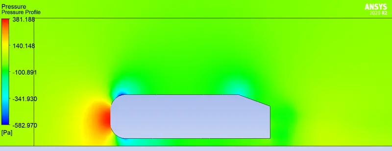
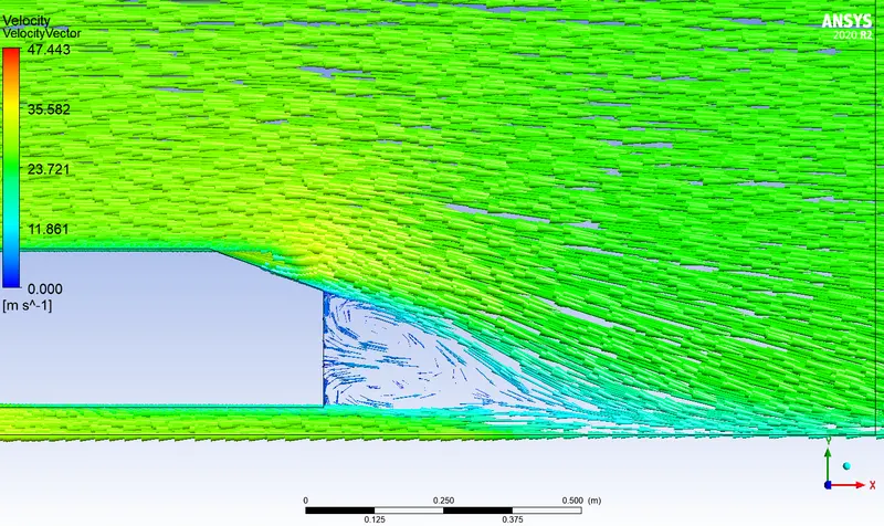
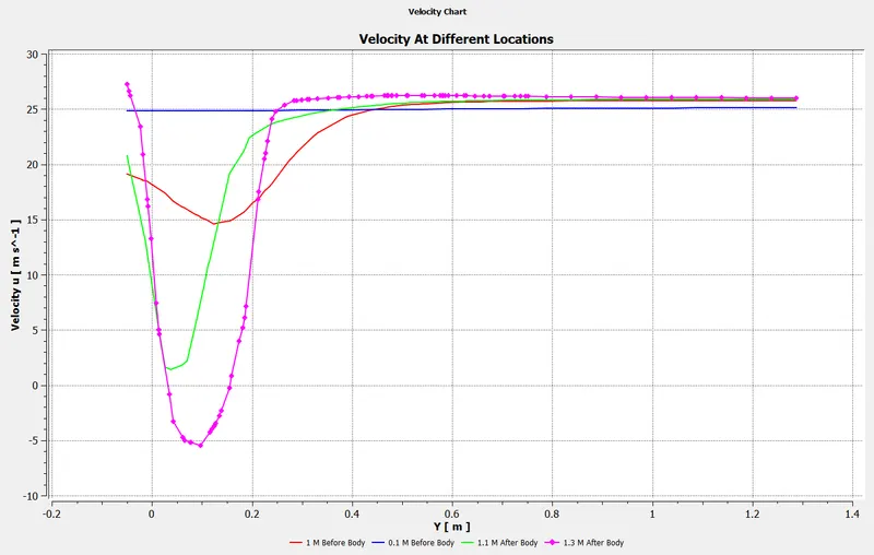
The post processing is required to study the results came from simulation. In post-processing all velocity and pressure contour with vector plot are used to study flow in wake region and point of separation from Ahmed body model. Another important aspect in the post-processing is getting the chart of velocity and pressure value in the domain. This is done by using line option and chart option in post-processor. The location has been considered before the body and after the Ahmed body. This will provide information on the velocity and pressure co-relation before and after flow region.

1) Residuals

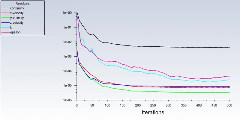
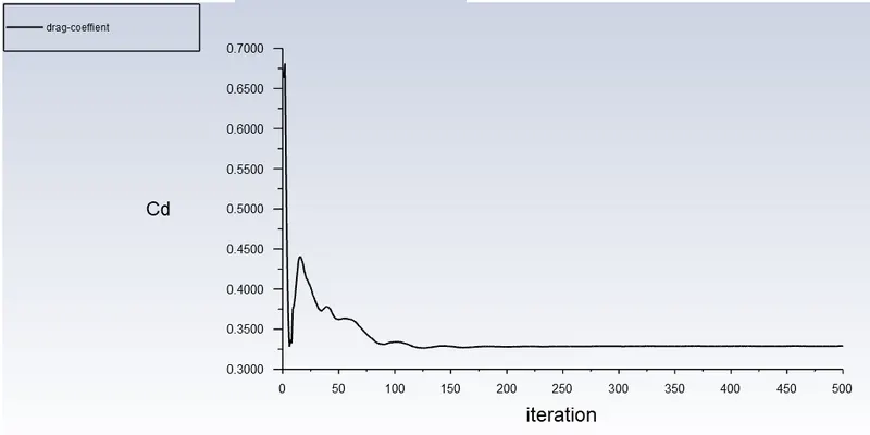
2) Coefficient of Drag

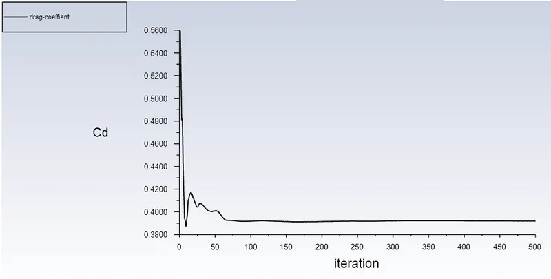
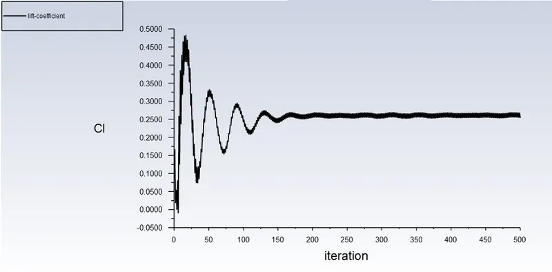
3) Coefficient of Lift

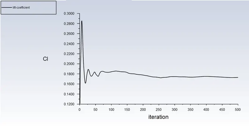
4) Velocity Contour

5) Pressure Contour

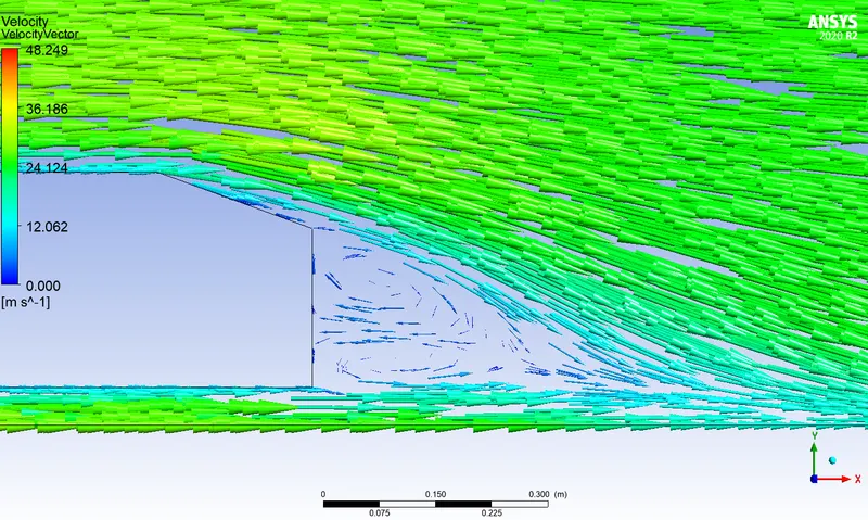
6) Vector plot

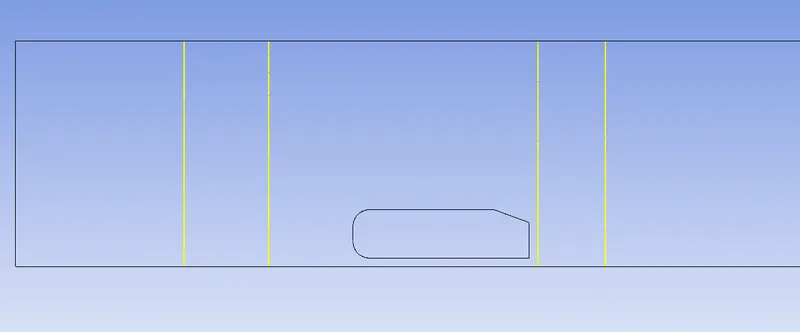
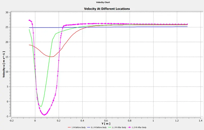
To get the chart at different location it is required to have line at that location which will take the data of velocity and pressure and plot it over value user wants. The location of lines are given below:

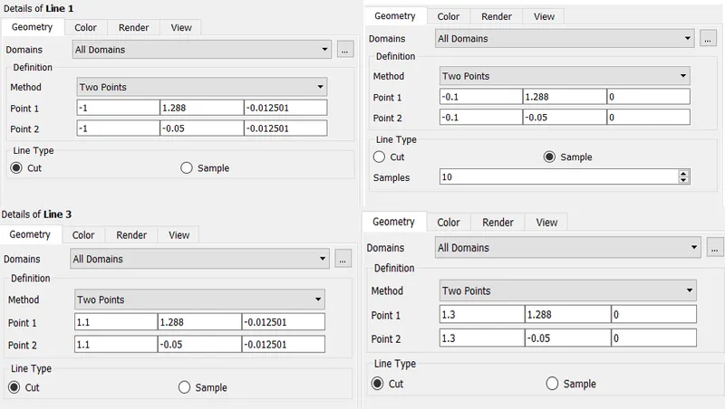
After providing this line location the graphic will show lines in the setup which is shown below

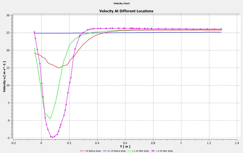
7) Velocity chart

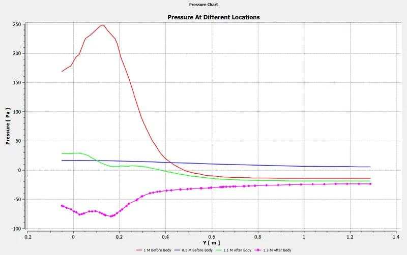
8) Pressure Chart

Case 2 – Mesh Setup

For case 2 mesh we are restricting our mesh size to 0.1m to all the components present in workbench. Also we are restricting our global face mesh size to 0.1m only. After applying this mesh parameters, the mesh will look like:

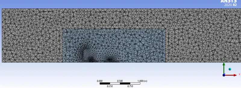
The number of element created in the mesh are 199295.

The rest of the thing will be same as baseline mesh setup; this simulation will also be run for 500 iterations.

Post-Processing (Case 2): -

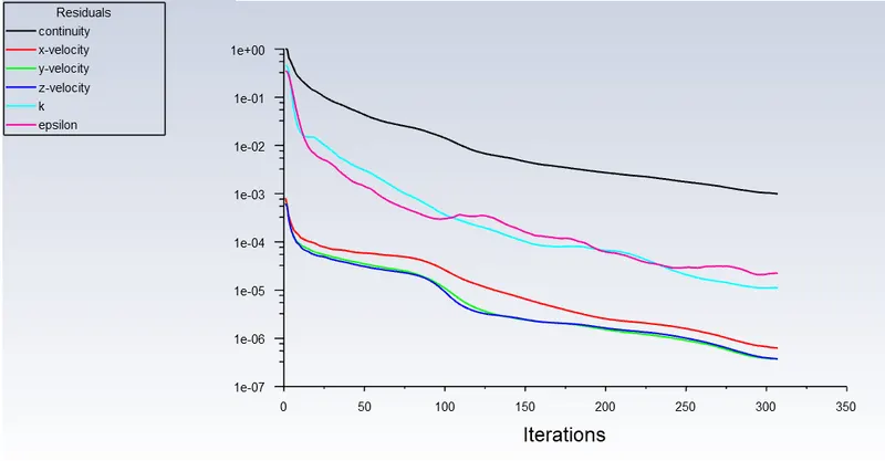
1) Residuals

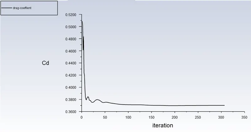
2) Coefficient of Drag

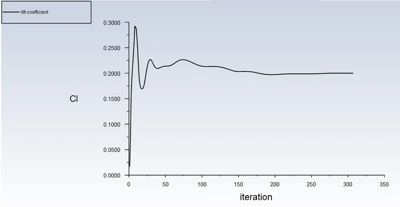
3) Coefficient of Lift

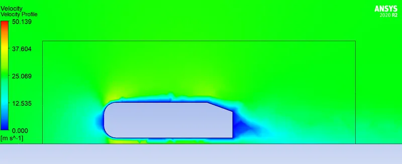
4) Velocity Contour

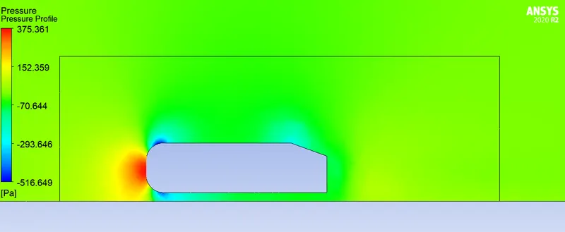
5) Pressure Contour

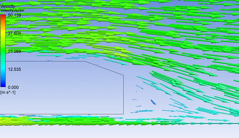
6) Vector plot

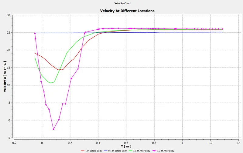
7) Velocity Chart

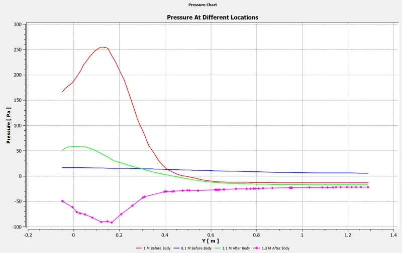
8) Pressure Chart

Case 3 – Mesh Setup

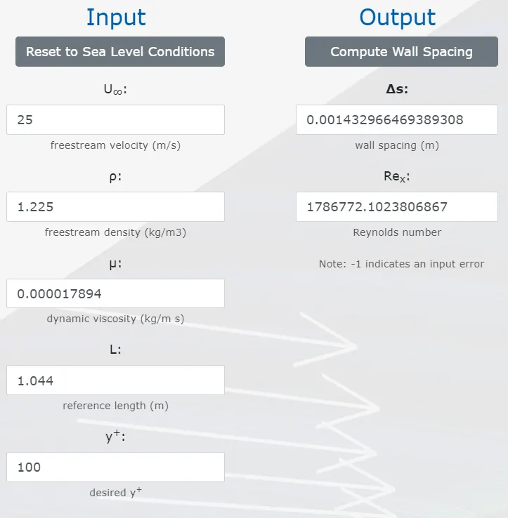
In case 3 we will be dealing with inflation layers. Inflation layer can be provided in global mesh setup or local mesh setup depending on the user requirement. In global mesh setup it is important to consider named selection for geometry whereas in local mesh setup user get more freedom for choosing named selection face or geometry selected faces. Before providing inflation layer it is important to calculate Y plus value for first layer thickness. For this mesh setup we are selecting desired Y plus value of 100 and layer of inflation will be 5 only. To calculate the first layer thickness we are going to use below formulas:

1 – Calculation of Reynolds Number

`Re=(ρVL)/μ=(1.225*25*1.044)/(1.789e^(-5) ) =1786772.10`

2- Calculation of skin friction coefficient

`C_f=0.026/(Re^(1/7) )=(0.026)/(1786772.10)^((1/7) ) =0.003325`

3- Calculation of Shear stress near wall.

`τ_(wall)=(C_f*ρ*U^2)/2=(0.003325*1.225*(25)^2)/2=1.2728 N/m^2`

4- Calculation of Friction velocity

`U_(Fric)= √(τ_(wall)/ρ )= √(((1.2728))/((1.225) ))=1.019`

5- Calculation of first layer thickness

`ΔS=(Y^+*μ)/(U_(Fric)*ρ) =((100*1.78e^(-5) ))/((1.019*1.225))=0.001433 m`

6- Total thickness of Inflation for 5 layer

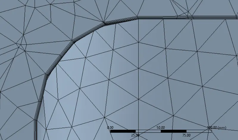
`Total ThickNess =1.433*((1.2)^5 )=3.56 mm`

The calculated value of the first layer thickness is 1.433 mm, if we compare this value with available Y plus calculator online we can get same results:

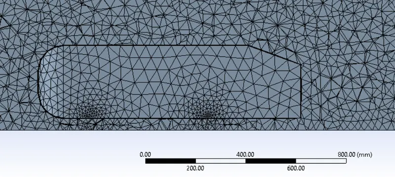
After providing the value in the mesh setup, the mesh will look like:

The enlarged view near car-wall is seen as:

The amount of element for the mesh is 298094.

The rest of the setup will be same for simulation. The results are given in post-processing.

Post-Processing (Case-3): -

1) Residual

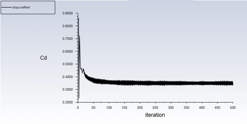
2) Coefficient of Drag

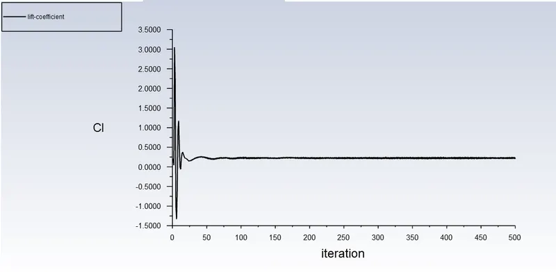
3) Coefficient of Lift

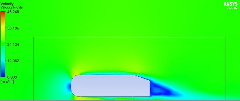
4) Velocity Contour

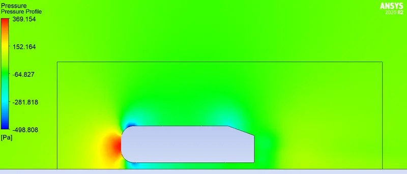
5) Pressure Contour

6) Vector Plot

7) Velocity Chart

8) Pressure Chart

Case 4- Mesh setup: -

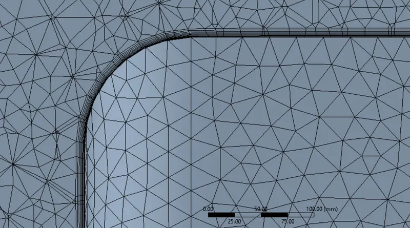
In this case we are using mesh value of 0.05m for outer enclosure and 0.025m for inner enclosure with 10 inflation layers. The total thickness of the inflation layer is 8.85mm. After applying the parameters, the mesh is shown below:

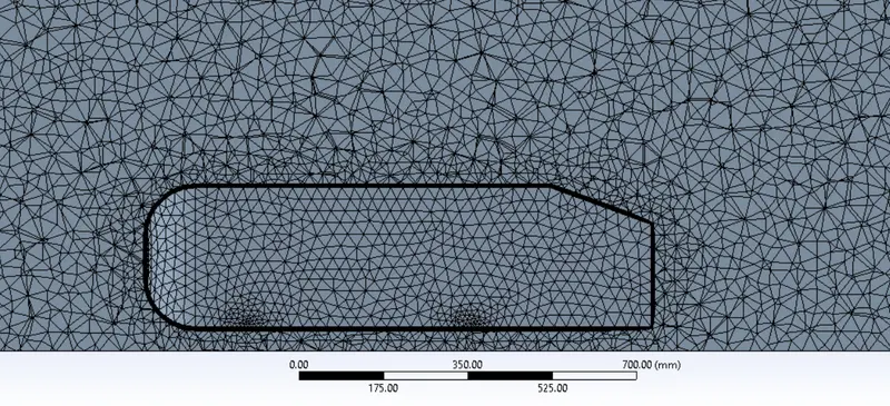
The amount elements created in the mesh are 379892. The inflation layer near body are shown below:

Post-Processing (case 4): -

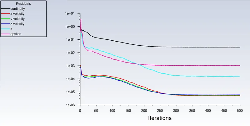
1) Residuals

2) Coefficient of Drag

3) Coefficient of Lift

4) Velocity Contour

5) Pressure Contour

6) Vector plot

7) Velocity Chart

8) Pressure Chart

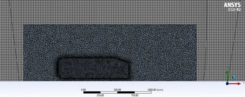
Case 5 – Mesh Setup

In this case we are using lower mesh size for both enclosures. For outside enclosure 0.025m mesh size and for inner enclosure car-wall body is 0.01m. The inflation layer will be same as case 4. After applying this parameter, the mesh will look like:

The expanded view near the wall of car is shown as:

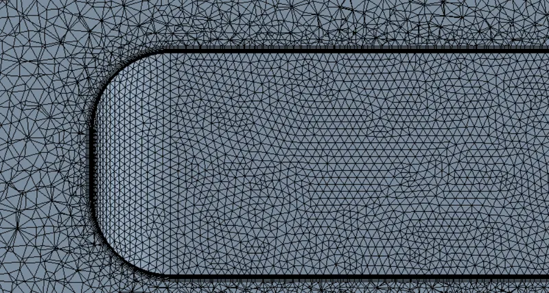
The amount of element created in the mesh are around 2424401. It is important to know that with lesser number of element the quality should be consistent. For this mesh size quality of mesh should be known, which is shown below.

1) Skewness Element Quality

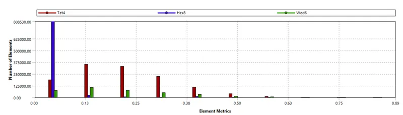
2) Orthogonal Mesh Element Quality

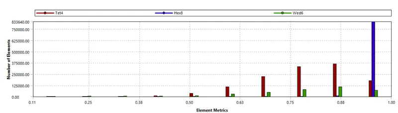
From the both element quality criteria it is evident that both quality control criteria are under acceptable condition and will provide better results in simulations.

Post-Processing (Case 5): -

1) Residual

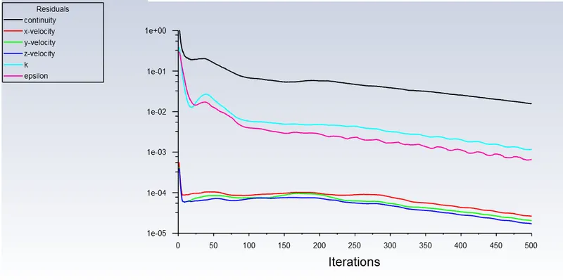
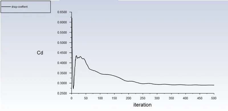
2) Coefficient of Drag

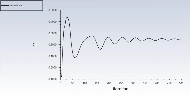
3) Coefficient of Lift

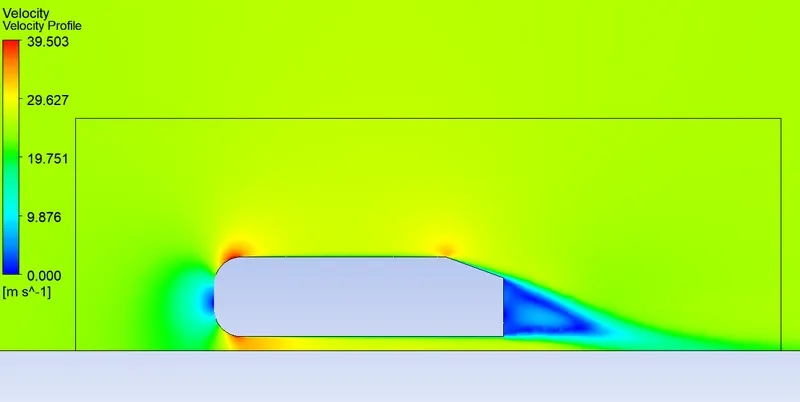
4) Velocity contour

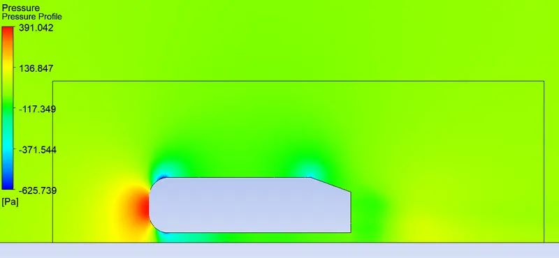
5) Pressure contour

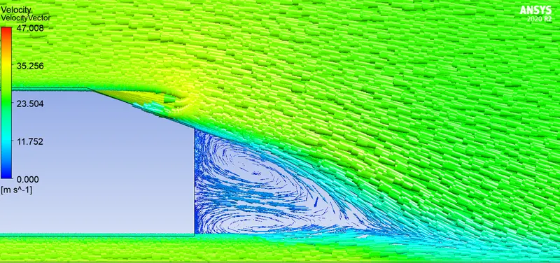
6) Vector plot

7) Velocity Chart

8) Pressure Chart

9) Velocity Gif

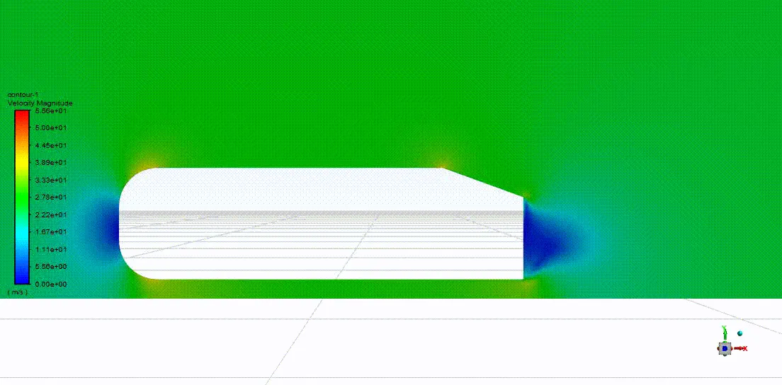
Table of Comparison

Parameters	No. of Elements	Coefficient of Drag	Coefficient of Lift
Case 1	80455	0.391	0.173
Case 2	199295	0.370	0.199
Case 3	298094	0.353	0.201
Case 4	379892	0.329	0.254
Case 5	2424401	0.314	0.261

Point of Separation in fluid flow:

The point of separation in boundary layer theory is one of the important aspect. As we know that Reynolds number is ratio inertia force to viscous force. When there is flow on the body the fluid layer close to the surface of body experienced high viscous force rather than inertial forces. Viscous force tries to adhere the body but eventually as the flow going further the inertial forces increase in dominance. A point come where this two net forces becomes zero is called separation point. Further of the point the negative pressure development has started near a wall of body but actual flow still flowing on the body which results in the separation of flow due to negative gradient.

This separation of fluid flow creates only adverse effect. As it goes further the streamline separation point create separation bubbles in the flow field and cause flow to stop and reattach at some distance in the flow, which can be seen as following image:

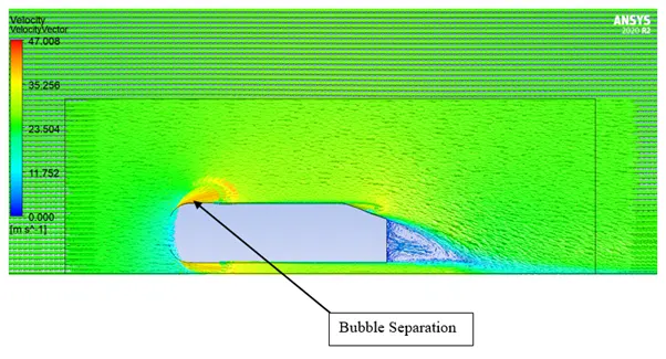
For the reattachment of fluid flow start again from zero and continue till negative gradient develops in the flow filed. The separation point also gives rise of vortices generation near the wall of fluid which are not suitable for fluid flow because of alternating frequency. If matched with structure frequency causes structural damage eventually. In every pressure contour of the simulation we can see the negative pressure development on the surface of Ahmed body which is indication of flow separations.

Negative Pressure in Wake Region

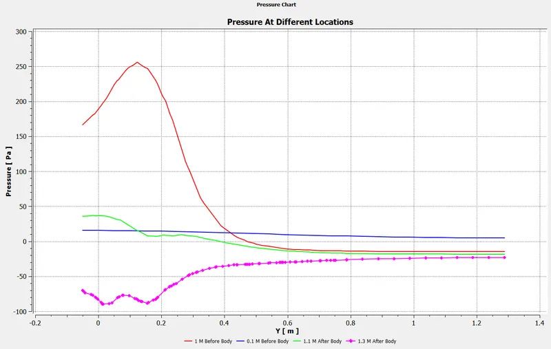
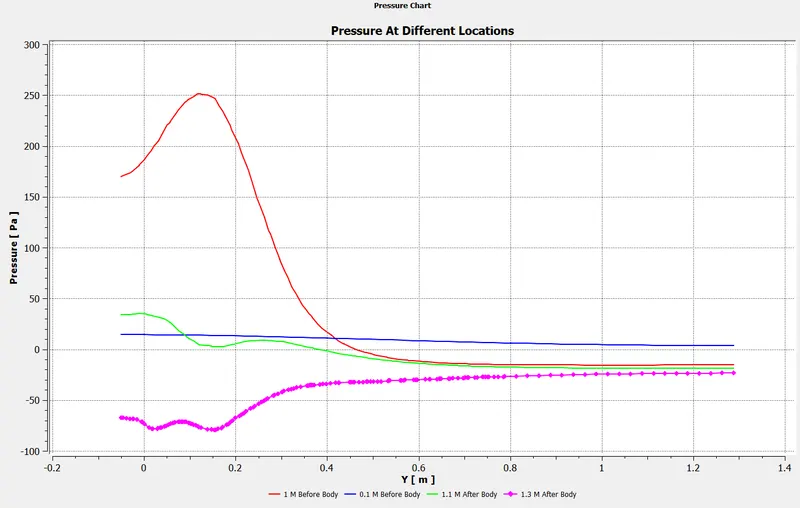
The negative created in the wake region is due to pressure difference between upstream flow and downstream flow. As we can see in the chart of pressure from case 5 simulation;

The green line is the plot behind the Ahmed body, the lower region of Ahmed body has low negative pressure value as compared to upstream region of Ahmed body. This is cause by mostly flow separation or adverse pressure gradient created during the flow. This cause creation of vacuum behind the Ahmed body which results in loss of performance in car also it creates pressure drag.

Conclusion: -

• From the simulation in each case we can found that as the mesh gets finer we are getting correct result near to accuracy. Also the coefficient of drag is decreasing and coefficient of lift is increasing in value.
• Case 4 and Case 5 provide more accurate result in the wake region when compared with rest of the cases. This is happening because of better mesh resolution near the boundary of Ahmed body.
• From the flow chart of velocity and pressure we can observe well suited plots when compared with experimentation value. The velocity before the body is higher as compare with region behind body because of wake generation where velocity becomes almost zero. Similarly, we can see the pressure gradient throughout the flow field.
• For mesh independent test we can say that case 4 gives overall better result also with less amount of computational effort. Inflation layer provide added advantage to capture the flow near the Ahmed body.
• The cause of flow separation in the fluid flow is because of negative pressure generation in the boundary layer of flow near wall of body and negative wake region is generated due to the pressure difference between low stream and high stream flow also due to flow separations.