Week 4 - Genetic Algorithm

Genetic Algorithm

Aim: -

Optimization of the equation to find global maxima by genetic algorithm using stalagmite function and explain the genetic algorithm working in MATLAB.

Objective: -

• To study the genetic algorithm working.
• To use the stalagmite function to calculate the global maxima.
• To make sure genetic algorithm comes up with correct value for each iteration.
• To plot the 3D graph for each study of genetic algorithm.

Description: -

In many of engineering problem optimization of working condition or to predict the certain problems higher and lower value is much more important. Using trial and error method for various iteration leads to unstable solution and provide the wrong maxima and minima. It also depends upon the problem how we are going to address in case of optimization. The use of genetic algorithm for the optimization problems or stochastic problem lowers the effort of user and predict the solution in less amount of time.

Genetic algorithm is very popular method to solve the stochastic problem and optimization problems. It was totally depending on the theory of evolution given by Charles Darvin. Genetic algorithm is one of the most stochastic algorithms often used to solve the large-scale optimizations problem in the various field. The genetic algorithm was first introduced by Holland (1975), is a powerful stochastic search algorithm based on a mechanism of natural genetic and selection. A general description of genetic algorithm is as follows:

1. The genetic algorithm starts with an initial set of Random solution called the populations. This population is depending on the series of number for which local or global maxima or minima is need to be find out.
2. Each individual in the population is called chromosomes which represents a solution to the problem at hand.
3. The chromosomes evolve through the successive iteration called the generations.
4. During each generation, the chromosomes are evaluated using some measures of fitness.
5. To create the new generation, new chromosome called offspring are formed by either merging two chromosomes from the current generation using a crossover operator or by modifying a chromosome using a mutation function.
6. A new generation is formed by either selecting according to fitness value some of the parents and offspring or by rejecting others so as to keep the population size constant.
7. Filter chromosome have higher probabilities of being selected. After several selection generations, the algorithm converges to the best chromosome, which hopefully represents the optimum or suboptimal solution to the problem.

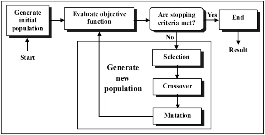
Genetic algorithm is differing from other regular algorithm in sense of sampling the points and converge to the optimal solution in less amount time. In regular algorithm the space and bounds are need to specify explicitly and the selection process is totally depending on the user requirement but in case of genetic algorithm the bounds and the selection process of parents and offspring are done by algorithm and it marching towards the solution according to best fit crossover or mutated value.

The genetic algorithm in the MATLAB comes with the special syntax and according to the solver, some of them are given below:

1. To find the local unconstrained minimum value of the function we need to use x = ga(fun,nvars) where ‘fun’ is function associated whose minimum value has to be find and ‘nvars’ is the number of variable in the equations.
2. To find the local minimum of x to the function when the linear inequality is present in the equations. The linear inequality is the point which is inactive when the solution of function is less than zero. To evaluate the value we need to use x = ga(fun,nvars,A,b) where A is the matrix function of b.
3. To find the local minima of x to the function when the linear equalities are exist then use the syntax as x = ga(fun,nvars,A,b,Aeq,beq), the ‘Aeq’ and ‘beq’ can be find out be taking the variable x to left hand side of equation. The coefficient of x will be ‘Aeq’ and the value to the right-hand side of equation will be ‘beq’. We can set A = [ ] and b = [ ] if no linear inequality is found.
4. To find the local minima of x to the function with upper and lower bounds for x the syntax will be given as: x = ga(fun,nvars,A,b,Aeq,beq,lb,ub) where ‘lb & ub’ are lower and upper bound value respectively. If there is no inequality and equality constraint then the syntax is written as x = ga(fun,nvar,[ ],[ ],[ ],[ ],lb,ub)
5. To fine the local minima of x to the function with specific option in ga solver then we have to use syntax as x = ga(fun,nvars,A,b,Aeq,beq,lb,ub,nonlcon,options). The options require specific name in order to execute the ga solver. There are various optimization options like constraint tolerance, Crossoverfcn, Fitness limit and Population size,etc. Depend upon optimization type by the user he can use any of the option.

Governing Equation:

The solution for the equation for which the global maxima value has to be found is given as:

`f(x,y)=f_(1,x) .f_(2,x) .f_(1,y) .f_(2,y)`

`f_(1,x)=(sin⁡(5.1πx+0.5) )^6`

`f_(1,y)= (sin⁡(5.1πy+0.5) )^6`

`f_(2,x)=exp⁡(-4 ln⁡(2)((x-0.0667)^2/0.64) )`

`f_(2,y)= exp⁡(-4 ln⁡(2)((y-0.0667)^2/0.64) )`

Code Explanation:

1. The code stared with inputs to create the domain of problem in which solution lies. It is done by taking value from 0 to 0.6 with 150 value it in and then two-dimension mesh is created by ‘meshgrid’ command. The number of cases is put to 50 for which loop will be going to carry out the solution.
2. In the other script stalagmite function is written to get the variable x and y in term of input_vectors 1 and 2 which is stored in the array F. which was later used in the main code afterward in the for loop.
3. The whole code is divided in three different section, in section one we are going to evaluate global maxima of problem using stalagmite function and then using genetic algorithm to find the value of global maxima. In second section we are going to use the bounded value to perform the genetic algorithm which is described in the genetic algorithm syntax point 4 and in the last section we are using optimization option to increase the population size of parents and offspring to make the convergence, which is describe in the genetic algorithm syntax point 5.
4. As we know the genetic algorithm is always minimize the solution of function but in our case, we need to find the global maximum of function which is simply done by introducing the -ve sign in the stalagmite function.
5. After each of the section we are plotting the results and using the ‘surfc’ command to create 3-dimensional view for global maxima.

The code for the genetic algorithm is given as:

1) Stalagmite Function

function [f] = stalagmite(input_vector)

x = input_vector(1);
y = input_vector(2);

f_1_x = (sin(5.1*pi*x + 0.5))^6;
f_1_y = (sin(5.1*pi*y + 0.5))^6;
f_2_x = exp(-4*log(2)*((x-0.0667)^2/0.64));
f_2_y = exp(-4*log(2)*((y-0.0667)^2/0.64));

% Use of -ve sign to change the minimum to maximum.

[f] = -((f_1_x)*(f_2_x)*(f_1_y)*(f_2_y));

end

2) Main code for Genetic Algorithm with statistical behaviour.

clear all
close all
clc

% Inputs for the domain 
x = linspace(0,0.6,150);
y = linspace(0,0.6,150);
num_case = 50;


% Creating 2D domain
[xx,yy] = meshgrid(x,y);

% Evaluating the Stalagmite Function

for i = 1:length(xx)
    for j = 1:length(yy)
        input_vector(1) =xx(i,j);
        input_vector(2) =yy(i,j);
        f(i,j) = stalagmite(input_vector);
    end
end

tic
% Section 1- Genetic Algorithm with Statistical Value without Bound Value

for p = 1:num_case
    [inputs,fopt_1(p)] = ga(@stalagmite,2);
    xopt(p) = inputs(1);
    yopt(p) = inputs(2);
end

Section1_Time = toc;

% Plotting for Section 1 Results
figure(1)
subplot(2,1,1)
hold on
surfc(xx,yy,-f)
shading interp
colorbar
plot3(xopt,yopt,-fopt_1,'marker','o','markerfacecolor','r','markersize',5)
title('GA with Unbounded Inputs')
subplot(2,1,2)
plot(-fopt_1)
xlabel('No. of Iterations')
ylabel('Maximum Value of Function')

3) Main code for Genetic Algorithm with Bounded value

clear all
close all
clc

% Inputs for the domain 
x = linspace(0,0.6,150);
y = linspace(0,0.6,150);
num_case = 50;


% Creating 2D domain
[xx,yy] = meshgrid(x,y);

% Evaluating the Stalagmite Function

for i = 1:length(xx)
    for j = 1:length(yy)
        input_vector(1) =xx(i,j);
        input_vector(2) =yy(i,j);
        f(i,j) = stalagmite(input_vector);
    end
end

tic
% Section 2- Genetic Algorithm with Bounded value

for p = 1:num_case
    [inputs,fopt_2(p)] = ga(@stalagmite,2,[ ],[ ],[ ],[ ],[0;0],[1;1]);
    xopt(p) = inputs(1);
    yopt(p) = inputs(2);
end

Section2_Time = toc

% Plotting for Section 2 Results
figure(1)
subplot(2,1,1)
hold on
surfc(xx,yy,-f)
shading interp
colorbar
plot3(xopt,yopt,-fopt_2,'marker','o','markerfacecolor','r','markersize',5)
title('GA with bounded Inputs')
subplot(2,1,2)
plot(-fopt_2)
xlabel('No. of Iterations')
ylabel('Maximum Value of Function')

4) Main code for Genetic Algorithm with bounded inputs and increased populations.

clear all
close all
clc

% Inputs for the domain 
x = linspace(0,0.6,150);
y = linspace(0,0.6,150);
num_case = 50;


% Creating 2D domain
[xx,yy] = meshgrid(x,y);

% Evaluating the Stalagmite Function

for i = 1:length(xx)
    for j = 1:length(yy)
        input_vector(1) =xx(i,j);
        input_vector(2) =yy(i,j);
        f(i,j) = stalagmite(input_vector);
    end
end

tic
% Section 3- Genetic Algorithm with Bounded value and Increased Iteration
options_1 = optimoptions('ga');
options_1 = optimoptions(options_1,'PopulationSize',289);

for p = 1:num_case
    [inputs,fopt_3(p)] = ga(@stalagmite,2,[ ],[ ],[ ],[ ],[0;0],[1;1],[ ],[ ],options_1);
    xopt(p) = inputs(1);
    yopt(p) = inputs(2);
end

Section3_Time = toc

% Plotting for Section 3 Results
figure(1)
subplot(2,1,1)
hold on
surfc(xx,yy,-f)
shading interp
colorbar
plot3(xopt,yopt,-fopt_3,'marker','o','markerfacecolor','r','markersize',5)
title('GA with bounded Inputs with Increased Interation')
subplot(2,1,2)
plot(-fopt_3)
xlabel('No. of Iterations')
ylabel('Maximum Value of Function')

Inference from plots: -

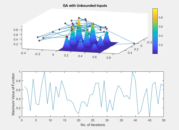
From the above plot as we can see, the genetic function calculates the random population on its own and creating its offspring and trying to make selection proper. But the search space is larger and making it very difficult for selection. In the second plot we can interpretate that it has all the random nature of value ranging between the 0 and 1.

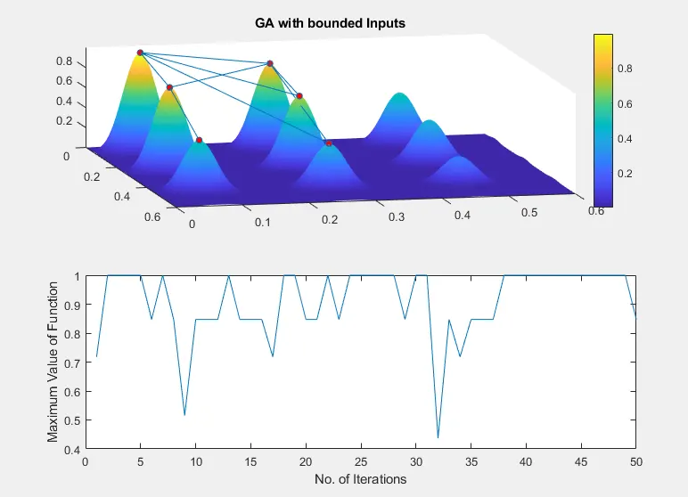
In the above graph, the genetic function is constrained in the bounded value whereas in former one it was choosing random value for selection. As we can see in graph that genetic algorithm using value from the nearer maxima of another tip. Also, in second graph we are seeing clear spike maxima value of function.

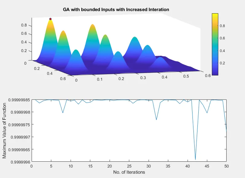
As we are seeing in above graph the genetic algorithm has successfully capture the maxima of function by increasing the population value using ‘PopulationSize’ options. In other graph as we can see the tip of maxima function has been iterate over 42 iteration. Making function bounded in the search and increasing population size increase the convergence ratio of genetic algorithm to select the best possible offspring of the created population.

Error faced during Coding:-

1) Error one.

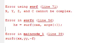
This error is caused due to providing wrong value in the stalagmite function. Because of error the surfc command was not working and it was corrected by re-checking every parameter in code and function.

2) Error 2

This error not because of any code mistake or spelling mistake while writing, it was error related to the version of MATLAB. For the third section calculation of genetic algorithm, the PopulationSize option was not taken into consideration. After going through the documentation for each of the version of MATLAB it was seen that, in optimization toolbox of MATLAB there are other solver and its seperate optimoption selection. In that section it found that MATLAB version 2015a is not support 'PopulationSize' option for genetic algorithm in any of the optimization solver. It was corrected by upgrading to the MATLAB version. Any version from 2016a will have the 'PopulationSize' option as per my reasearch.

To check whether the 'optimoption' works or not, go to command window and search for:

>> doc OPTIMOPTIONS
>> 

Conclusion: -

The genetic algorithm is used successfully to capture the maxima of function but in actual practice it use to minimization of function. For each section genetic algorithm makes the population and select approprite parent and offspring, and also try to create the new generation on the basis of cross-over and mutation. As the population size increase the amount of time taken to converge to the required output will get increase. In case of section 3 where the population size is increased by 289 it took 31.3664 second to complete the solution whereas for the section 2 it has taken only 9.3460 seconds.

References: -

1) https://in.mathworks.com/help/gads/ga.html

2) https://www.youtube.com/watch?v=6aacc_deEOQ&t=1482s

3) https://in.mathworks.com/help/gads/options-in-genetic-algorithm.html