Week 5 - Curve fitting

Curve fitting & Correctness of Curve

Aim:

Use of curve fit to predict the data of temperature and specific heat using linear and cubic polynomial.

Objective:

• To study the curve fit using python.
• To study the smoothness of curve-fit.
• To code the curve fit of given data.
• To plot the graph for each curve-fit data.

Description & Governing Equation:

The curve fit is the series of data we use to predict the given data how it will perform in nature. It is the mathematical method to predict data afterward if not stored or provided. To fit the data, we use many mathematical equations to select the data near to the actual datapoints. Curve fitting involve either interpolation, where an exact fit to the data is required or smoothing in which a smooth function is constructed and approximately fits the data.

Curve fit include the how much data is associated with actual datapoints and how much is the error while using certain equation to match the actual data. The smoothness of curve is mostly depending on the error which we are getting. The order of polynomial will take care for the best fit available for actual data. We can use either polynomial function or square function depending upon the user requirement or else we can have our own equation to satisfy the curve fit.

The goodness of fit is which already discussed can be characterized in four different way:

• The sum of squares due to errors (SSE)
• R square
• R square adjusted
• Root mean square error (RMSE)

All of this goodness of fit can be explained by an example in which we consider the certain data set with total variability as explained variability and unexpected variability. If we consider the specific heat as total variability then temperature is the explained variability on which specific heat traced with error as unexpected variability.

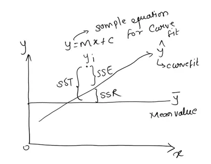
As we can see in above figure, we are assuming a function to fit the data. Y^hat is the curve fit value and Y bar is the mean value of the predicted data set. Then we can represent the equation as:

Total sample variability = Explained variability + Unexplained variability

Which can be renamed as per our need as:

Specific heat variability = Air temperature + other factors or errors

Which is equals to:

SST = SSR + SSE

Where,

SST = Total sum of squares.

SSR = Sum of square of regression.

SSE = Sum of square due to errors.

The SSE which we defined as the sum of square due to error is most probably calculated using least square method which is given as:

`SSE=(Y_(i )- hatY )^2`

The R square method is used to measure how successful is the fit in explaining the variation of data. It is the relation between predicted value of dataset to the original value of dataset. The R square value is given as:

`R^2= (SSR)/(SST) or 1-((SSE)/(SST))`

Where,

`SSR=(hatY - barY )^2`

And

`SST=(Y_i- barY )^2`

The Adjusted R square error will be depending upon the how many variables are there in the curve fit equation. Adding the new variable in the equation will eventually increase the accuracy or goodness of curve. Also depending upon how the added variable significant and insignificant it will relate to the fit. It can be calculated as:

`R_(adj)^2=1- [((1-R^2)(N-1))/(N-K-1)]`

Where,

N = Number of datapoints.

K = The number of Independent variables.

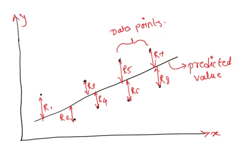
The Root Mean Square Error is the standard deviation of residuals. These residuals are the difference between the datapoints and curve-fit model which we have used. So, having lower value of RMSE means the datapoints are near to the curve-fit value which is desirable in any curve fit.

Code Explanation: -

1) The code started with importing important modules such as numpy, matplotlib and scipy. The scipy module is necessary for solving curve fit problem unlike MATLAB in which curve fit module is directly as a toolbox.

2) The curve fit function is created by using linear polynomial and nother function is created with the cubic polynominal. This function are later used in the code for curve fit.

3) To plot the temperature and cp from the file it is required to read the file first. This is done by defining another function of read file with name of file and the 'r' reading instruction. As the file contain two value separated by ',' hence the line split function is used to saperate the two value. And each of the value is read and stored in separate arrays.

4) For linear curve fit, from the function of reading file, temperature and Cp is read. Then curve fit function is used for normal or actual data and then same linear function is used to curve fit the next data.

5) Similar to linear curve fit, cubic polynomial is used to fit the data for temperature and Cp.

6) After curve fit, the methods are used to measure the fitness of curve for both linear and cubic curve fit.

The program for curve fit is given below:

"""
Week 5 Challenge - Curve fit for Temperature and Cp
Written By: Shubham K. Chaudhari
Date : - 28 August 2021
"""
import math
import matplotlib.pyplot as plt
import numpy as np
from scipy.optimize import curve_fit

#Linear Curve fit Function
def function_L(t,a,b):
    return a*t+b
# Cubic Curve fit Function
def function_C(t,a,b,c,d):
    return a*pow(t,3)+b*pow(t,2)+c*t+d

# Reading Temperature and Cp from data file
def read_file():
    temperature = []
    cp = []
    for line in open('data','r'):
        values = line.split(',')
        temperature.append(float(values[0]))
        cp.append(float(values[1]))
    return [temperature,cp]

# Linear Curve fit Program
temperature,cp = read_file()

popt, pcov = curve_fit(function_L,temperature,cp)
fit_cp_L = function_L(np.array(temperature),*popt)
plt.figure(1)
plt.plot(temperature,cp,'--',color = 'blue',linewidth = 3)
plt.plot(temperature,fit_cp_L,color = 'red',linewidth = 3)
plt.legend(['Pre-Curve fit data','Linear Curve fit Data'])
plt.xlabel('Temperature in Kelvin')
plt.ylabel('Coefficient of Heat')
plt.title('Linear Curve fit Plot')
plt.show()

# Cubic Curve Fit Program
popt,pcov = curve_fit(function_C,temperature,cp)
fit_cp_C = function_C(np.array(temperature),*popt)
plt.figure(2)
plt.plot(temperature,cp,'--',color = 'blue',linewidth = 3)
plt.plot(temperature,fit_cp_C,color = 'red',linewidth = 3)
plt.legend(['Pre-Curve fit data','Cubic Curve fit Data'])
plt.xlabel('Temperature in Kelvin')
plt.ylabel('Coefficient of Heat')
plt.title('Cubic Curve fit Plot')
plt.show()

"""
Measuring Fitness of Curve fit using:
SSE - Sum of Error Squared
SSR - Sum of square of Regression
SST = SSE + SSR
R^2 = SSR/SST
RMSE = (SSE/l)^0.5
where l is the total size of function for which curve fit is done
"""

s = np.sum(cp)
l = np.size(cp)
m = s/l
print('Mean Value of Cp',m)
print('')

# Fitness for Linear Curve fit
sse_linear = 0
ssr_linear = 0
for i in range(l):
    error_linear = abs((np.sum((cp[i]-fit_cp_L[i]))))
    sse_linear = sse_linear + pow(error_linear,2)
    ssr_linear = ssr_linear + np.sum(pow((fit_cp_L[i]-m),2))
print('Measure of Fitness for Linear Curve fit')
sst_linear = sse_linear + ssr_linear
print('SST Linear',sst_linear)
R2_linear = ssr_linear/sst_linear
print('R2 Linear Fit',R2_linear)
RMSE_linear = pow((sse_linear/l),0.5)
print("RMSE Linear fit",RMSE_linear)
print('---------------------------------------------------------------------------------------')

# Fitness for Cubic Curve fit
sse_cubic = 0
ssr_cubic = 0
for i in range(l):
    error_cubic = abs((np.sum((cp[i]-fit_cp_C[i]))))
    sse_cubic = sse_cubic + pow(error_cubic,2)
    ssr_cubic = ssr_cubic + np.sum(pow((fit_cp_C[i]-m),2))
print('Measure of Fitness for Cubic Curve fit')
sst_cubic = sse_cubic + ssr_cubic
print('SST Cubic',sst_cubic)
R2_cubic = ssr_cubic/sst_cubic
print('R2 Cubic Fit',R2_cubic)
RMSE_cubic = pow((sse_cubic/l),0.5)
print("RMSE Cubic fit",RMSE_cubic)
print('')

Inference of Plot:

1) Curve fit for Linear degree of Polynomial.

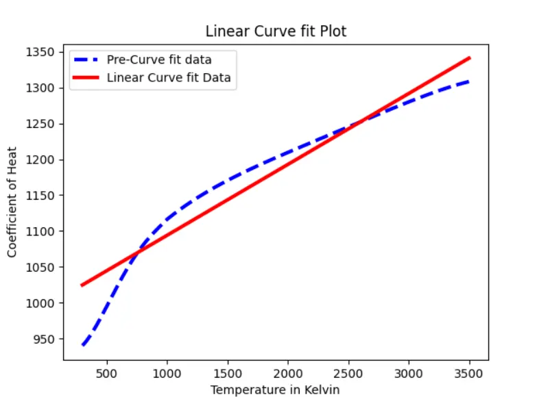
From the above graph as we can see that there is more deflection between the original curve shown in blue line and predicted curve for 1st order polynomial fit which is shown in red. On the left side is the Y axis of specific heat and at bottom there is x axis of temperature in kelvins.

2) Curve fit for Cubic degree of Polynomial.

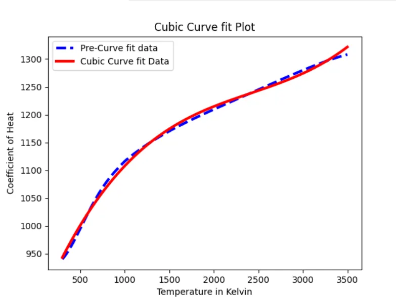
From the above graph if we compare to the 1st order polynomial curve it seem better and the error is less. The predicted value is matched for the most of datapoints of orignal curve.

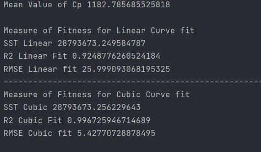
From the above output console, it can be seen that fitness of curve for R2 is near to 1 for cubic is nearer as compared to linear curve fit. Similar to R2, RMSE measure of curve fit for linear fit is around 26 and for the cubic fit is 5. Whatever nearer to 1 will have best of fit to actual values.

Question 1: - What does popt and pcov mean?

Answer: - 'popt' means the representation of matric which stores and extract the coefficient for value fitting according to equation defined.

'pcov' represent the square matrix which store the estimated values of covariance of the coefficient of above. The diagonal element of this square matrix also represent variance of coefficient.

Question 2: - What does np.array(temperature) do?

Answer: - This command convert each value of temperature in the data file into in array using numpy.

Question 3: - What does the *in *popt mean?

Answer: - *popt it indicated and returns the value of each coefficient stored in popt array.

Question 4: - What need to be done in order to make the curve fit propertly?

Answer: - From the curve fit data it is seen that for linear polynomial there is big difference between the curve fitted Cp and actual Cp, whereas when cubic polynomial is used there was lowerest error is found. To make the actual fit rather using polynomial equation, quadratic equation can be also used or the degree of coefficient can be increased.