Week 4.1: Project - Steady state simulation of flow over a throttle body
Week 4.1 Challenge – Steady State Simulation of flow over throttle body
Aim: - Steady state simulation throttle valve inside the pipe with difference in pressure.
Objective: -
- To study the importance of throttle valve in flow simulations.
- To set up the steady state simulation for throttle valve.
- To create the embedding mesh near to throttle valve for better convergence.
- To post process the results from the simulation.
- To plot the graph of pressure, mass flow rate and velocities.
Introduction: -
To regulate the flow inside the pipe and to maintain the pressure across the domain throttle valve are used. This valves are operated manually or automatically through sensors and actuators. The application of throttle valve is seen in engine to actuate flow inside the cylinder and maintaining it according to applications. In engine the flow of coolant is also regulate by the butterfly valve which is one of the throttle valve in action. The throttle valve assembly is inserted between the two pipes where they are joined.
Solution Methodology: -
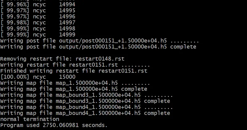
The steady state simulation is setup for this problem. The geometry comprises of throttle valve inside and it is in three-dimension structure. As it is a flow simulation the thickness of pipe is not required. For this simulation, the rotation of throttle valve is not required because of steady state simulation does not allow to rotate the valve for cycles. In converge studio the pre-processing is done for creating domain for fluid inside the pipe. The patch option is used to create the closing face for inlet and outlet. The simulation is run for 15000 cycles.
Pre-Processing: -
- Geometry
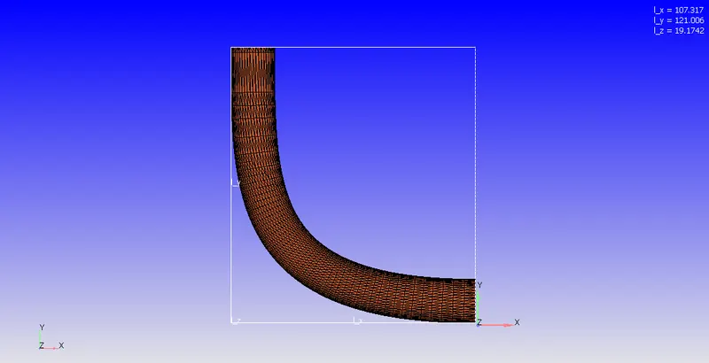
The geometry is imported directly in the converge studio by drag and drop method. The geometry is in the millimeter by default but the converge work in SI unit hence it is required to scale the geometry in meters.
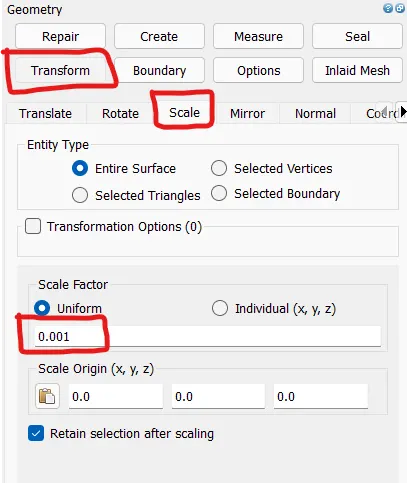
Using the geometry transform option in which scale tool is used to convert the dimension into meters. The scale factor is 0.001 is applied.
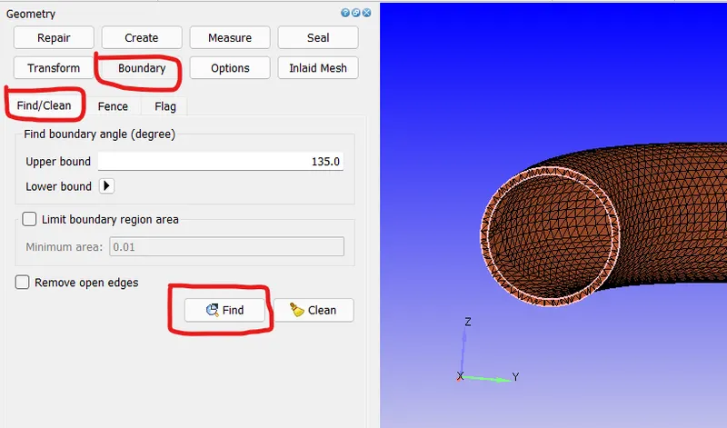
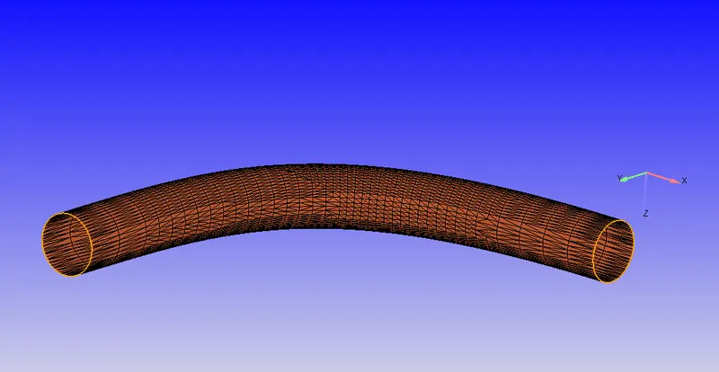
After completing the scaling of the geometry, it is required to clean the geometry by closing the flow domain. This is done by finding the boundary with open faces.
As it stated earlier, the thickness of body is not required for the simulation. Hence the outer faces of the body are need to be deleted. Similarly, the faces with open edges need to be patched. This can be done using hotkeys after selecting the face by angle options. Or user can go to repair tab in which delete option can be used to delete the specific face in geometry.
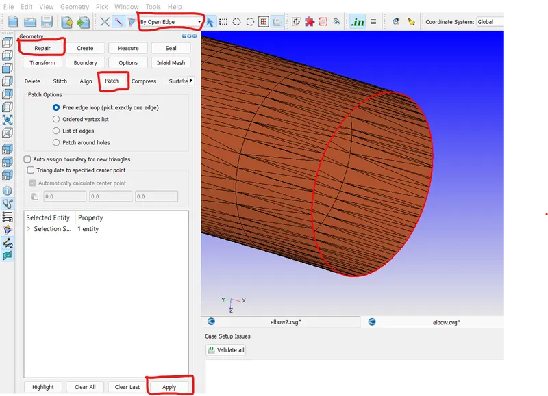
After deleting the surface which are not required for the simulation, it is necessary to patch the open faces. This can be done using the open edge option in the selection toolbar which only allows to select the open edges present in the geometry. The patch option can be find out from the repair tab in which patch option present. The patch option capture the open edge and connect it with creating a face. This has to be done on the both side of elbow to make it as inlet and outlet face.
2. Boundary Creation
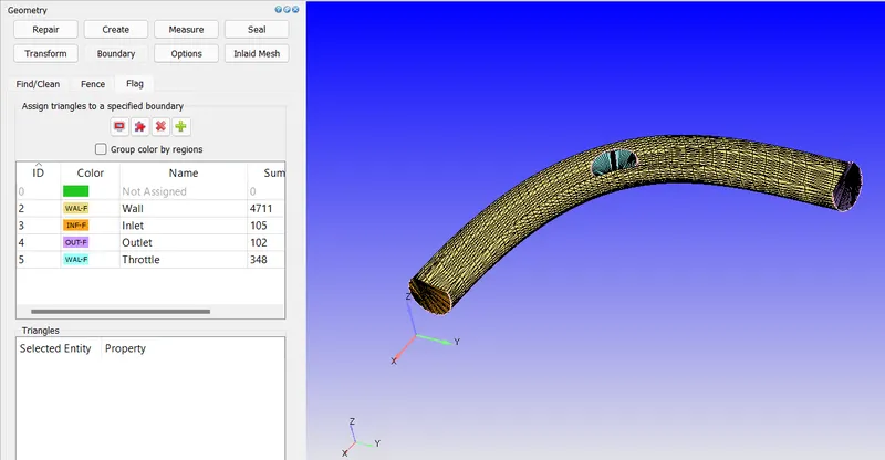
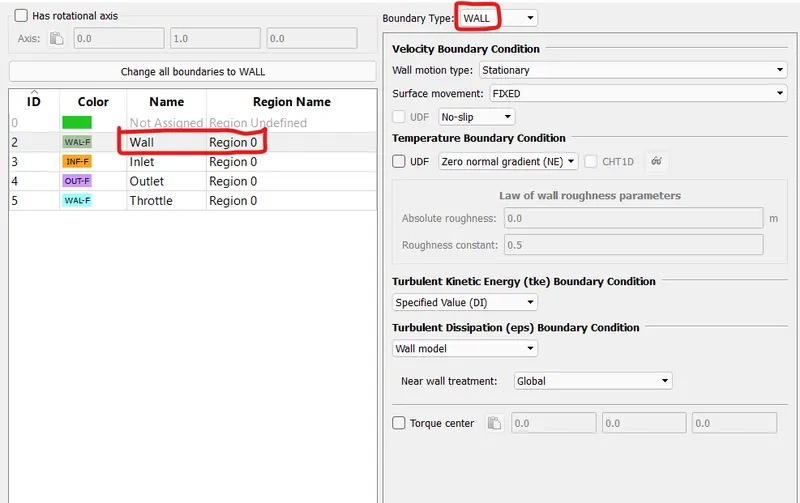
The creation of boundary in the converge studio is the main aspect to for meshing the geometry. As converge use mesh free method like cut cell meshing, it requires enclosed geometry for successful operation. The boundary creation is done in the boundary tab of the geometry setup section in which flag option is used. Four boundary are created in the setup which are wall, throttle, inlet and outlet. The wall is selected as elbow outer space, throttle is selected as the body inside elbow. The selection of body inside elbow can be done by hiding elbow after assigning to the boundary which make only throttle and other faces to be seen. After this the remaining two faces can be selected as inlet and outlet.
3. Case Setup
A) Type of Application of Simulation
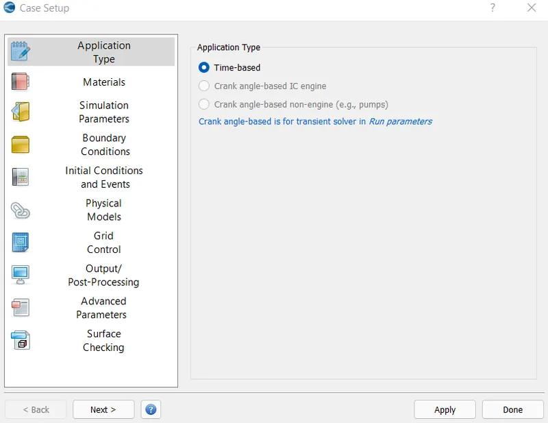
The simulation type for the problem is steady state but for the converge studio it is treated as time marching problem. Later in the solver type it can be changed.
B) Material type
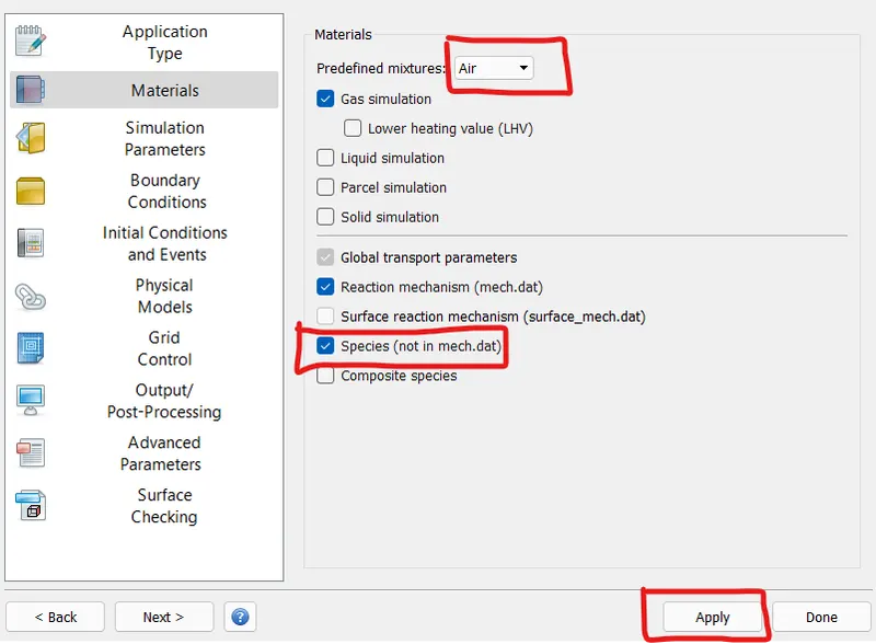
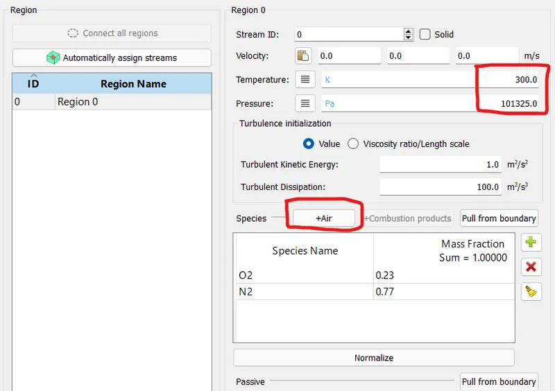
The fluid for the simulation is simply Air without considering the species input file as it was not required.
C) Simulation Parameter
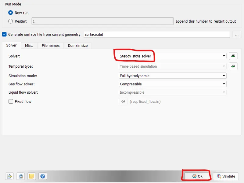
The solver setup is being set up to steady state with simulation mode with as full hydrodynamics. The gas flow solver is consider as compressible in nature.
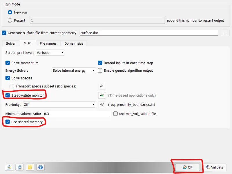
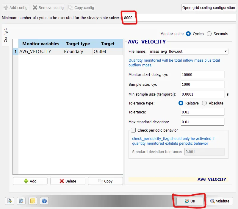
In the same case, for miscalleneous tab it is necessary to turn on steady state monitor for convergence purpose. The simulation can be performed without steady state monitor but it will run for whole process which is a waste of time.
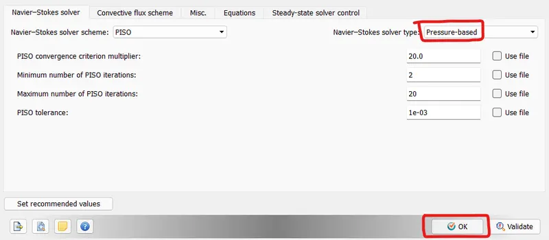
The simulation will be treated as pressure based approach as the velocity of the flow is very low. The Navier-Stoke pressure velocity scheme is consider as PISO as it mostly work for irregular mesh with better convergence.
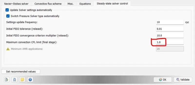
In steady state approach it is important to set the solver setting to automatic and the switching of pressure solver type to automatically so that any changes in the results or the solver process can be carried out efficiently. The CFL number for this simulation should be lower to 1 or 1. As it is a implicit solver it is unconditionally stable but the accuracy of the solution has to be consider while selection of CFL number.
As in steady state solver setup, the steady state monitor has been checked up hence it is necessary to create an steady state monitor for the simulation. This steady state monitor, monitors the solution and converge with the given parameter from user.
D) Boundary Conditions
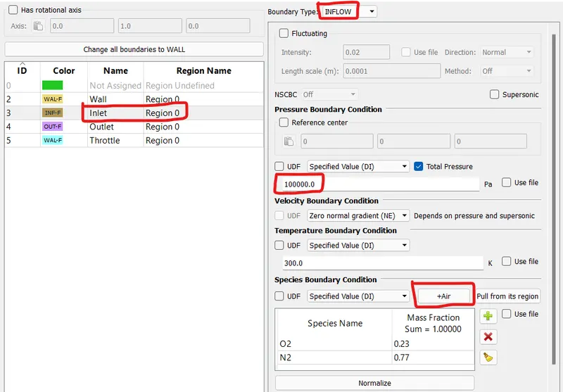
i] Inlet
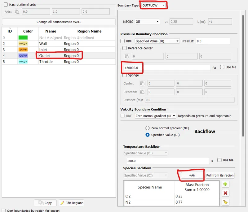
ii] Outlet
iii] Wall Elbow
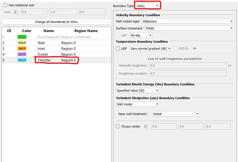
iv] Wall Throttle
In this case of steady state simulation there is no need of rotating the throttle valve because of conditions. The steady state simulation aims for the flow across the standard pressure and velocity without any changes in the geometry. Hence the throttle valve is consider as the normal valve in the domain
E) Initial Conditions and Region
For the PDE to solve, it required intial conditions and boundary conditions. For this problem pressure and temperature are consider as initial conditions. In the convege studio it is necessary to create the region before assigning the boundary conditions because in the boundary condition one has to select the region associate with respective boundary conditions hence it is better practise. The air has to be taken into consideration for the region of interest for the simulations.
F) Meshing
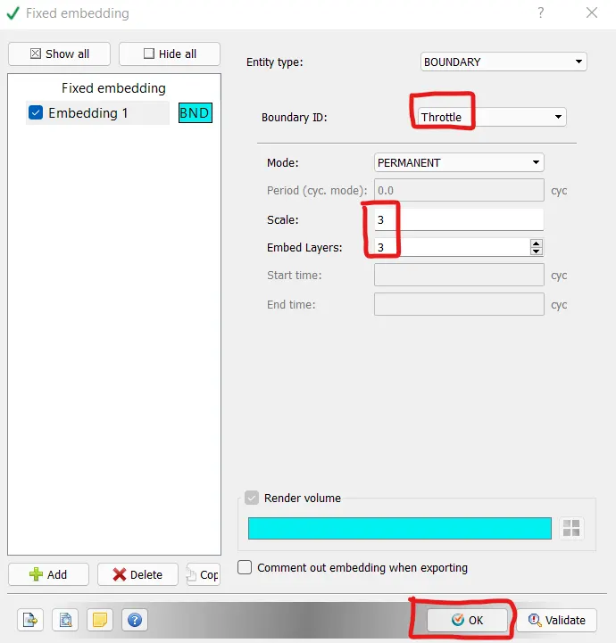
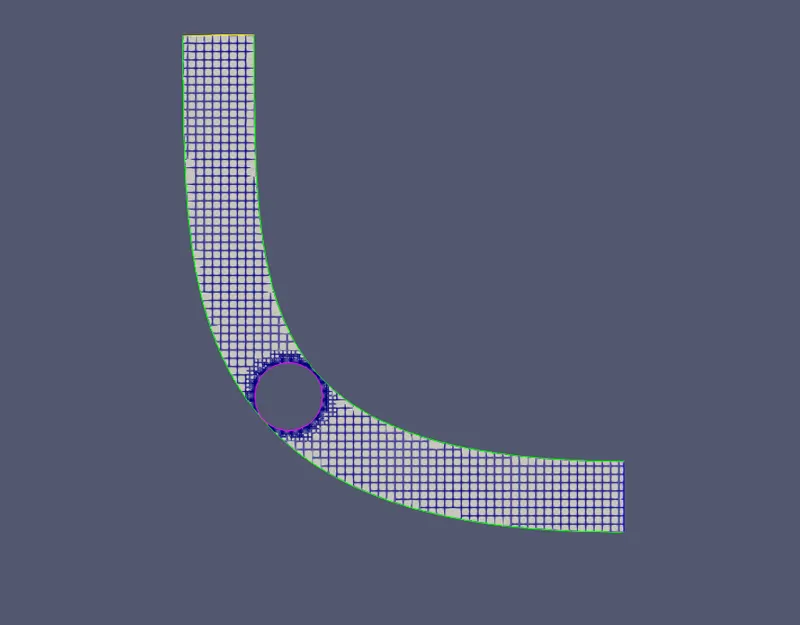
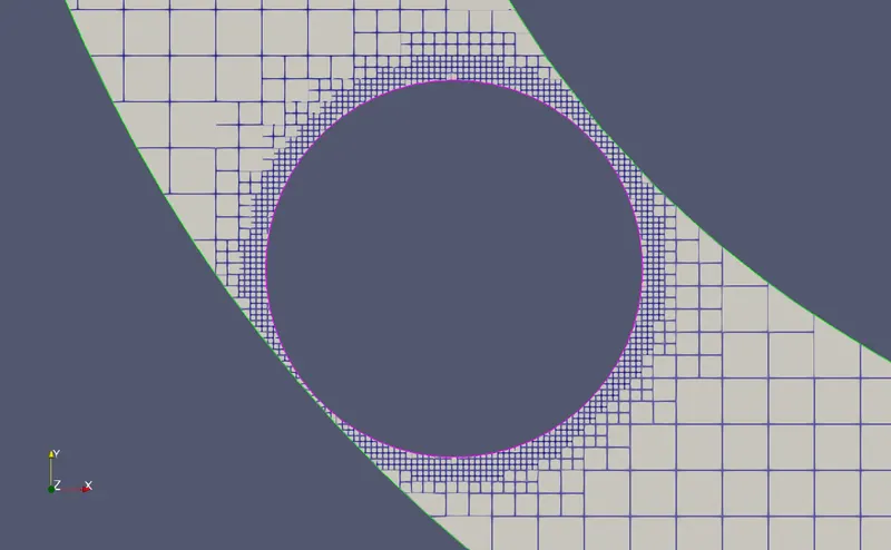
The meshing parameter for the problem is consider as 2mm. The area near the throttle is slender, to capture the flow parameter near the throttle valve it is necessary to create more number of element. This can be done by creating embedding mesh in the region near throttle valve. The parameter for embedding is given below:
G) Output files
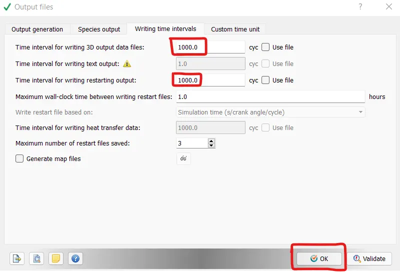
The creation of output file are important for the writing the 3D files which can be post-process in the paraview. The output control should be in such a way that, the solution should reach to steady state with enough number of output files to process.
4. Solution
The solution of problem can be start using Cygwin application in which command 'mpiexec.exe -n 8 converge.exe restricted' is used to excute the simulation. The 8 represent the number of processor used in the simulation.
5. Results
1) Mesh in Simulation
2) Mesh Near the Throttle Valve
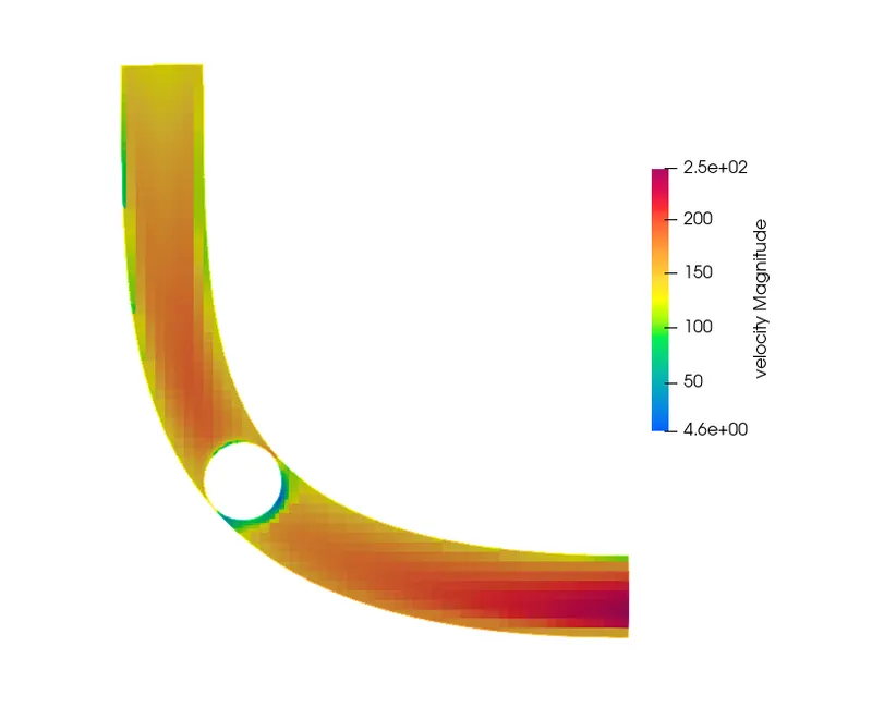
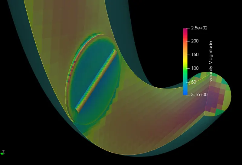
3) Velocity Contour
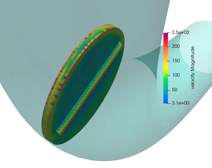
4) Velocity Near throttle
5) Velocity Contour 2
6) Pressure Contour
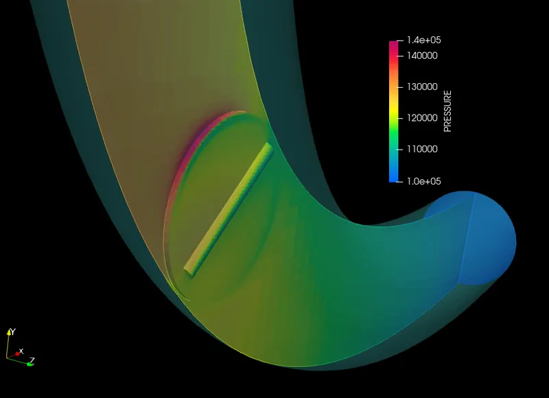
7) Pressure Contour 2
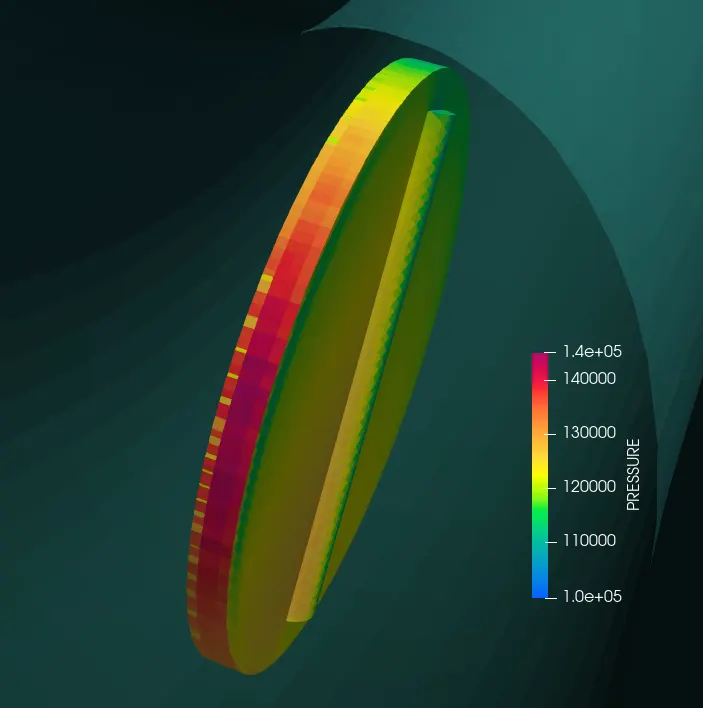
8) Video Animation of Pressure Contour
9) Video Animation of Velocity Contour
10) Pressure Plot
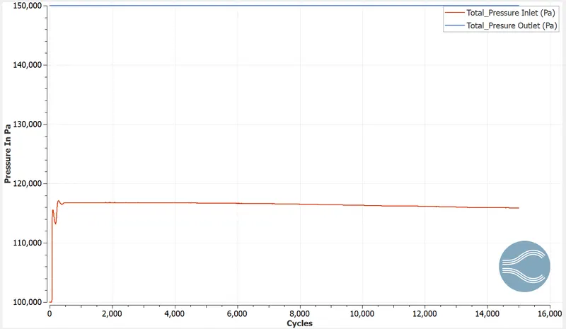
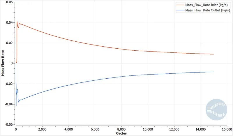
11) Mass flow rate
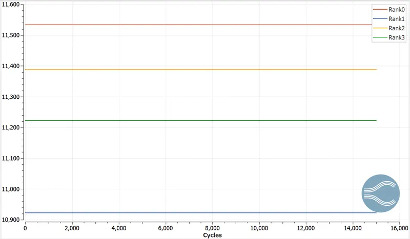
12) Total Cell Count
13) Time taken for Simulation
Conclusion: -
1) From the plot we can see that, mass inflow and outflow are opposite to each other providing information conservation of mass.
2) There is initial turbulence was seen on the throttle valve and later it has been converge.
3) The energy restriction is been provided by the throttle valve hence the increase in velocity is seen after the valve in flow field.