Week 8 - Simulating Cyclone separator with Discrete Phase Modelling

Aim: - Simulation of Cyclone Separator with Discrete phase monitoring method in ANSYS FLUENT.

Objective: -

• To study the working principle of cyclone separator.
• To study methods of separation efficiency of cyclone separator.
• To perform the DPM simulation of cyclone separator using anthracite as particle media.
• To perform the simulation by varying the particle size from 1 micrometer to 5 micrometer keeping velocity as 3 m/s.
• To perform the simulation by varying the velocity of flow from 1 m/s to 5 m/s keeping particle size constant of 5 micrometers.
• To compare the results of separator efficiency and pressure drop from the simulations.

Introduction: -

Cyclone Separator

Cyclone separator are inertial separation device which used the principle of inertia to remove the particulate matters from the gases. It is all known that particulate matter from 1 micrometer to 5 micrometers are not supposed to release in the atmosphere because of public health issue. Many industries where refineries are available use the cyclone separator before releasing the gases to the atmosphere. Cyclone separator are one of the many air pollution regulating devices which is known as precleaners as they remove the larger fragments of particular matter.

The cyclone separator can provide the both fine and larger particle separation. Cyclone separator can be made in single separator or multiple one which called as multicyclone which operates in parallel way. The size and height of the cyclone separator are depending upon type of gases passing through the machine.

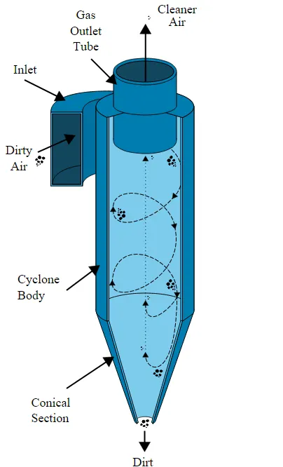
The cyclone separator is working on the principle of centrifuge but with the continuous supply of flue gases. In cyclone separator the dirty flue gases are fed into the chamber. The chamber is designed in such a way that the flow should in swirling motion. This swirling motion are as similar to the spiral vortex just like the tornado. The finer particles in the flue gases have less inertia which get influenced by the vortex motion of flow and tends to move upward from which gas outlet tube is present as shown in figure above. On the other hand, larger particular matter has more inertia and does not get more influenced by the vortex motion hence tends to move downward from conical section to dirt settling section of cyclone separator. Since the larger particle have more difficulty to cope with the swirling motion of gas and the vortex, the larger particle then hit the walls of container and then drop down to the hopper. The shape of chamber is upside down cone to influence the collection of bigger dirt particle in the hopper. Most of the cyclone are made and build to control and remove the particulate matter which is larger than 10 micrometers in diameter. However, there are more efficient cyclone which removes the particle size of 2.5 micrometers. Cyclone build for smaller particle size are not effective for the particle size more than 5 micrometers, for greater particle size rather than using cyclone separator it is better to go with gravity settling chambers and momentum separators. The general applications of the cyclone separators are oil refineries, cement industry and vacuum cleaners.

Cyclone separator are most probably able to remove the particular matter between 50-99% in the flue gases. The working efficiency of this cyclone separators are mostly depending upon the size of particles. If the flue gases contain more less size particles, because of this less particle get separated out from cyclone separator. Cyclone separator works better for large particular matters despite of lower efficiency for lighter particles. The main advantage of having cyclone separator is because of less expensive to install and maintain as they have no moving parts.

Cyclone Separator Efficiency: -

• Lozia and Leith Model

Lozia and Leith model are the modification of Barth model version. The Barth model is developed on the basis of force balance. This model assumes that particle governed in the vortex flow are under the influence of two forces which are 1. centrifugal flow Z and 2. flow resistance W. The collection efficiency for the particle diameter d_pi can be calculated from the empirical relation as:

`η_i=1/(1+(d_pc/d_pi )^β )`

where β is an expression for slope parameter derived based on the statistical analysis of experimental data of cyclone with D = 0.25m given as:

`β=0.62-0.87 ln⁡(d_pc/100)+5.21 ln⁡(ab/D^2 )+1.05 [ln⁡(ab/D^2 ) ]^2`

and d_pc is the 50% cut size given by Barth

`d_pc= [(9μQ)/(πρ_p z_c v_((tmax) )^2 )]^0.5`

where core length Zc and core diameter dc are given as:

`Zc=(H-S)-[((H-S))/(D/B-1)][(d_C/B)-1] , d_c>B`

`Zc=H-S`

`d_c=0.47D (ab/D^2 )^(-0.25) (D_e/D)^1.4`

• Li and Wang Model

The Li and Wang model includes particle bounce or re-entrainment and turbulent diffusion at the cyclone separator wall. A two dimensional analytical expression of particle distribution in the cyclone is obtained from the given model. This model is based on the assumption of radical particle velocity and the radial concentration profile are not constant for uncollected particle within the cyclone also boundary conditions with the consideration of turbulent diffusion coefficient and particle bounce re-entrainment on the cyclone separator wall are given as:

`c= C_θ,at θ=0`

`D_r (∂c)/(∂r)=(1-α)ωc , r=D/2`

The expression for the collection efficiency for the particle of any size is given as:

`η_i=1-exp⁡{-λθ_1 }`

where

`θ_1=2π ((S+L))/α`

• Koch and Licht Model

Koch and Licht model is recognized the most common aspect of cyclones inherently turbulent nature of cyclones and the distribution of gas residence times within the cyclone. This model described the particle motion in the entry and collection region based on assumptions which are:

• Tangential velocity of a particle is equal to the tangential velocity of the gas flow i.e. there is no slip in the tangential direction between the particle and the gas.
• The tangential velocity is related to the radius of cylinder by µR = constant.

A force balance and an equation on the particle collections yields the grade efficiency is given as:

`η_i=1-exp⁡{-2 [(G τ_i Q)/D^3 (n+1)]^(0.5/(n+1)) }`

where `G= (8K_c)/(K_a^2 K_b^2 )`

`n=1- {1-(12D)^0.14/2.5} {(T+460)/530}^0.3`

`τ_i= (ρ_p d_pi^2)/(18μ)`

G is a factor related to the configuration of the cyclone and ƞ is related to the vortex and τ is the relaxation term.

• Lapple Model

Lapple model was developed based on the force balanced without considering the flow resistance in cyclone separator. It was assumed by Lapple that a particle entering the cyclone is evenly distributed across the inlet opening. The collection efficiency is 50% when the particle travels from the inlet half width to the wall in cyclone. The empirical relation to calculated given by Lapple for 50% cut diameter is given as:

`d_pc= [(9 μ b)/(2πN_e v_i (ρ_p- ρ_g ) )]^0.5`

where Ne is the number of revolution which is given by:

`N_e= 1/a [h+ (H-h)/2]`

The efficiency of collection of any size of particle is given by:

`η_i= 1/(1+ (d_(pc))/(d_(PI) ) ^2 )`

Solution Approach and Methodology: -

The simulation will be carried in the two part in first one the diameter size of particulate matter will be changed with constant velocity and in second one particulate matter size will be constant and velocity is varying. The approach toward the problem is simple as velocity of flow is not greater than Mach number. Hence approach will be pressure based solver with steady state conditions. There is no requirement of considering the solid geometry of cyclone separator as there in no requirement of erosion on metal surface due the flow of particulate matter. The pre-processing only includes volume extraction from the geometry and meshing with structured element for better accuracy from solution. In order to provide better meshing control over the volume proximity and curvature size functions are used in simulation. The problem comprises of one inlet and two outlets, one for escape of gas and other one for trapping particle at bottom of cyclone separator.

The methodology for problem is divided in two different parts which has been discussed earlier. The DPM changes will be minimal in first part whereas for part two particle velocity has to be in match with inlet velocity of cyclone separator. There are 10 case setup for whole simulation five for each parts.

Part 1: - Change of Particle size with velocity keeping constant.

Case 1 – Particle size 1micrometer with velocity of 3m/s.

Case 2 – Particle size 2micrometer with velocity of 3m/s.

Case 3 – Particle size 3micrometer with velocity of 3m/s.

Case 4 – Particle size 4micrometer with velocity of 3m/s.

Case 5 – Particle size 5micrometer with velocity of 3m/s.

Part 2: - Change of velocity with particle size keeping constant.

Case 6 – Particle size 5micrometer with velocity of 1m/s.

Case 7 – Particle size 5micrometer with velocity of 2m/s.

Case 8 – Particle size 5micrometer with velocity of 3m/s.

Case 9 – Particle size 5micrometer with velocity of 4m/s.

Case 10 – Particle size 5micrometer with velocity of 5m/s.

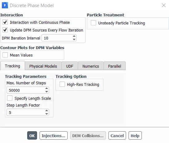
The case setup for each of the simulation will be same with some minute changes in the particle size and inlet velocity of particle and flow. It is important to consider some change in DPM which will eventually effect the separator efficiency. The changes are DPM iteration interval and maximum number of steps for calculation of tracking parameters. This changes will greatly affect the solution of tracked particle at the bottom of cyclone separator and can be discussed further in report.

Part 1: - Case 1 Setup

Geometry: -

The geometry of cyclone separator is in step format. The pre-processing work which need to be carried for the simulation is to remove the fluid volume from the geometry. This will be done by volume extract option in space-claim. The original geometry is showing below:

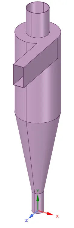
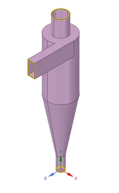
From the geometry it can be seen that, it is hollow and volume can be extracted for the simulation. The volume extraction is done by edge extract method which provide better results than rest of the option in the space-claim. It comes handy with geometry having inlet and outlet with closed edges and faces. Any defect in the geometry results in creation negative volume which could affect the simulation in drastic way. It is common practice to first check the geometry with any missing faces and missing edge and always try to stich the geometry before proceeding any extraction of volume or making an enclosure on geometry. The edge extract method is shown below:

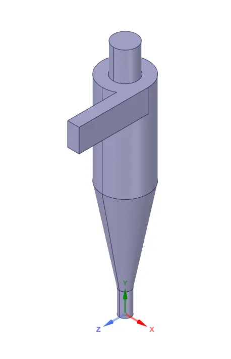
After the application of edge extraction on the geometry the final extracted volume will look like:

Meshing: -

After completing the extraction of fluid volume the meshing need to done for calculation of governing equation on the cell volume. The mesh which is used for the simulation is tetrahedron elements with size function. The initial mesh which is created in the meshing is kind of combination of bigger elements and smaller one. The original mesh created in ANSYS workbench is patch conforming without any size function. As there is very minimum edge of 2mm this create unbalance of mesh element near the where section of top outlet is start. The initial size of 5mm is taken into consider for simulation and minimum size function for element is 0.02mm for consideration of lowest edges. The mesh of geometry is showing below:

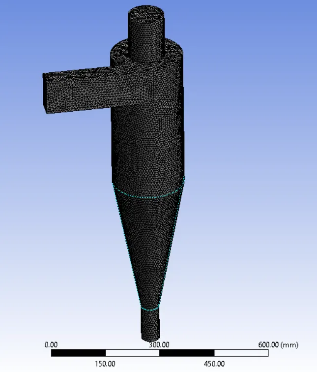
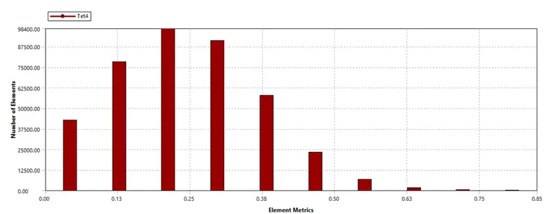
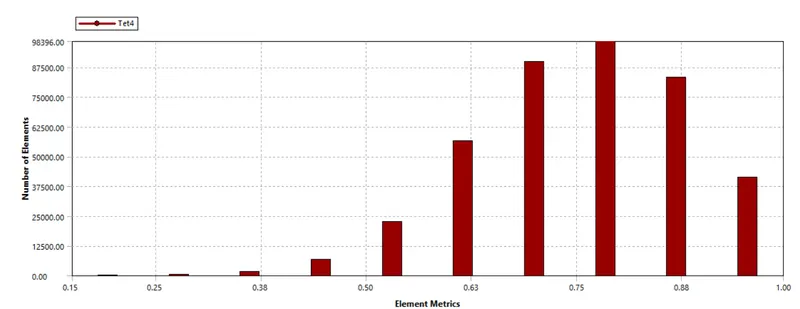
The number of element created in the meshing are 399096 and the number of nodes are 80810. The quality of mesh such as skewness and orthogonal quality are given below:

Skewness quality:

Orthogonal quality:

FLUENT SETUP

After successful transition of mesh from workbench to FLUENT it is important to first make the named selection for geometry so that boundary conditions can be defined accordingly. The named selection is shown below for geometry.

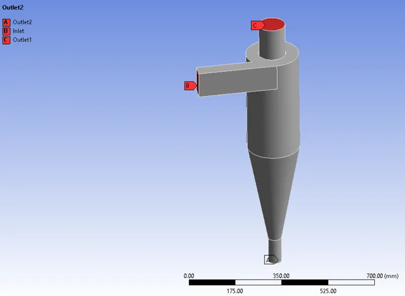
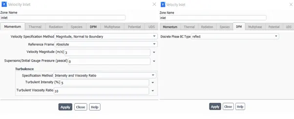
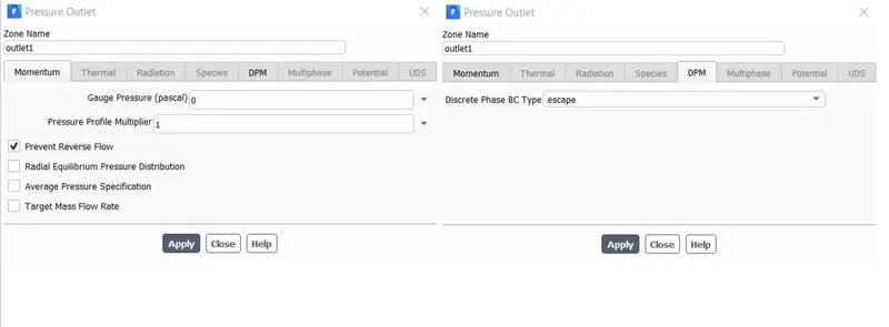
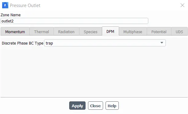
The named selection outlet1 is for the top opening and outlet2 is for the bottom collector. To calculate the pressure drop in the system we need to consider the top outlet as boundary condition for discrete phase is escape whereas for the bottom outlet it is trap condition. The general setup of FLUENT is very straight forward as it a steady state simulation and there no compressibility in flow pressure based solver can be used. The gravity is marked checked for providing gravity effect in the governing equation. The general setup for case 1 is shown below:

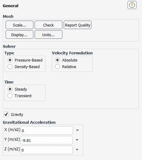
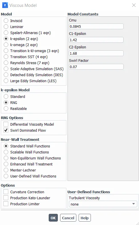
For turbulence model k-epsilon model with RNG model for swirl dominant flow. The viscous model for problem is shown below:

The other viscous flow parameter for particle which going to be in flow with air can be define in discrete phase monitoring option. In this option it is necessary to couple the particle results with normal flow. Iteration for every particle flow is need to be updated this can be activated in the same option. The DPM option is shown below:

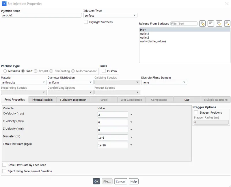
To define the particle for flow parameter the injection has to be created for simulation. Injection is method to insert the particle with respect to flow. The location of injection is irrespective of location of inlet for many simulations. The injection of particle can be group or single depend upon the flow requirement. It is not necessary that every particle should be just flowing with the primary liquid. The interaction between the particle and flow can be changed. Similarly, particle can make erosion on the surface of solid if consider into simulation. For this simulation the injection is consider as surface which means particle are injected with respect to the mesh at the surface. The surface which is used for injection is inlet of the problem i.e. primary flow is mixed with anthracite particles. The mass of the particle is considering as inert and diameter for first case is consider as 1micrometer with total flow rate is negligible. The velocity of particle is kept constant for first part of simulation which is 3 m/s. The particle injection is shown below:

Boundary condition: - Inlet

Boundary condition: - Outlet top

Boundary Condition: - Outlet bottom

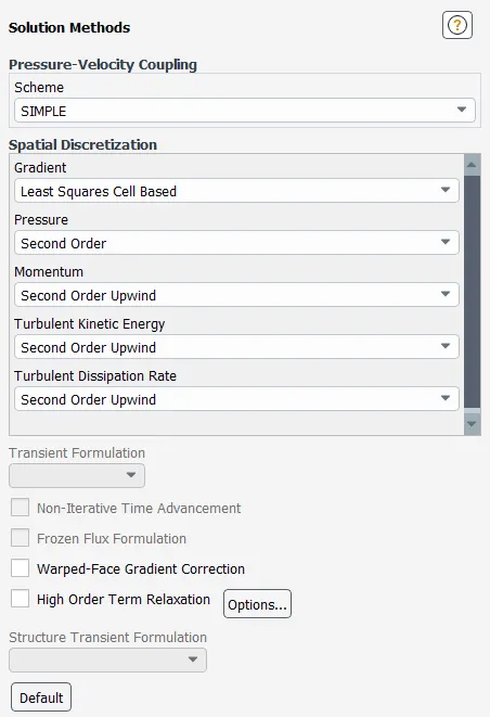
The solution method for the simulation are kept usual with some changes in turbulent dissipation and turbulent kinetic energy calculation. The pressure can be set as standard or PRESTO depend upon the user. From the initial guess it is better to go with standard discretization. The pressure-velocity coupling is considering as SIMPLE as it is mostly suited for steady state condition with pressure-based solvers. The image for solution method is shown below:

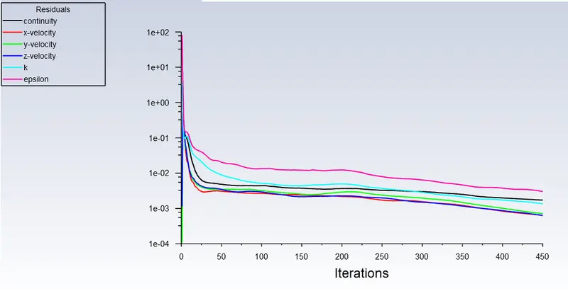
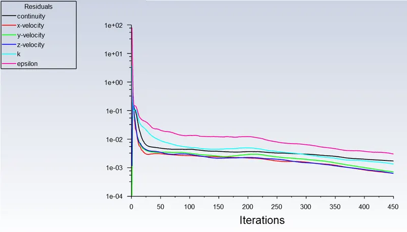
As the case come up with standard inlet and outlet it is better to go with standard initialization method before iterating the problem. After initialization the solution is run for in between 400 to 500 iterations. This has to be done to get max out of particle flow.

Result case 1: - (Particle Size = 1µm Velocity = 3m/s)

1) Residuals

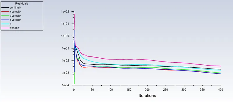
2) DPM Iteration result

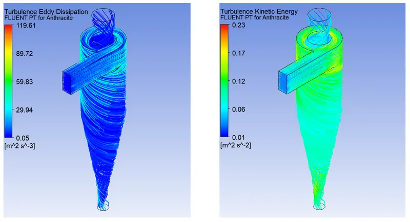
3) Turbulent Eddy dissipation and Turbulent Kinetic energy

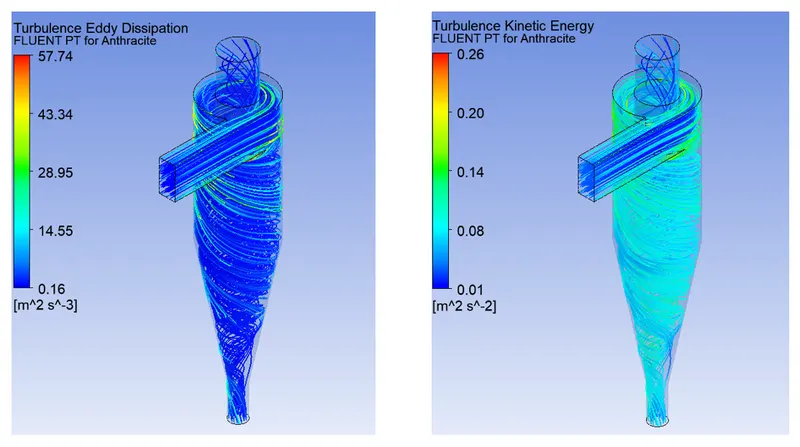
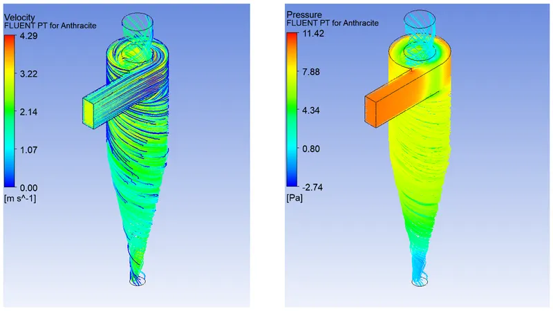
4) Pressure and Velocity

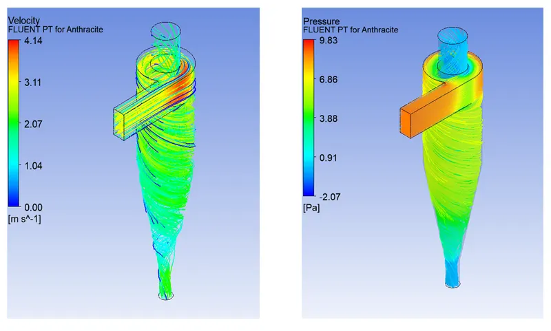
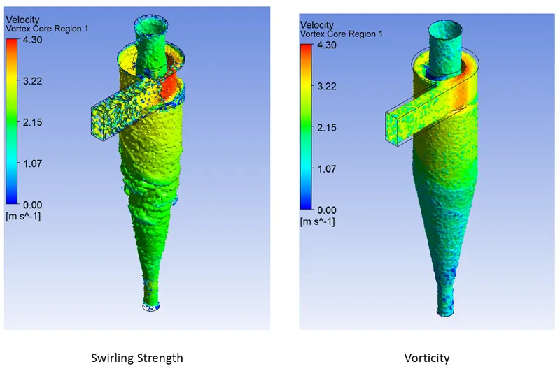
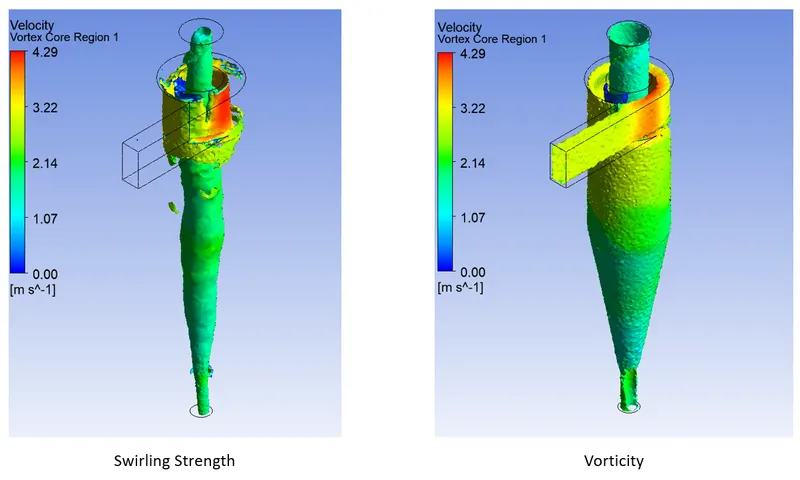
5) Swirling strength and Vorticity of Velocity

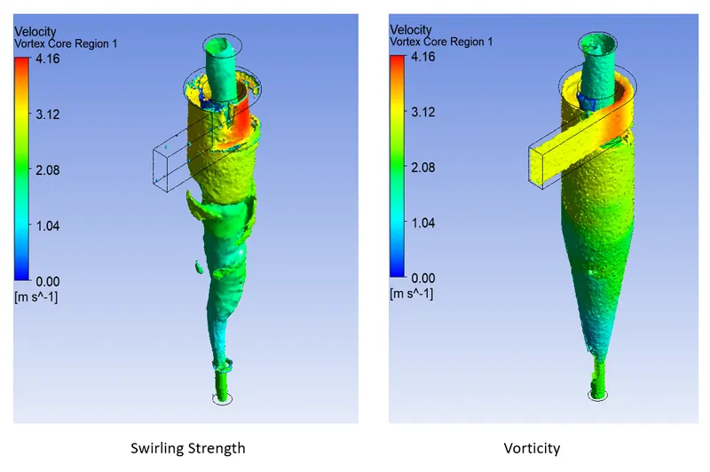
6) Separation efficiency

• Separation efficiency

The separation efficiency is defining as the ratio of the particle trapped at the bottom of the hopper to particle tracked from the inlet of cyclone separator. In this case the particle tracked are 300 and particle trapped are 78.

7) Pressure drop

The pressure drop for the system is calculated from inlet pressure and outlet pressure. The pressure should be total pressure from this both inlet and outlet.

`∆P=P_i-P_o=8.79-1.67=7.12 Pa`

Result case 2: - (Particle Size = 2µm Velocity = 3m/s)

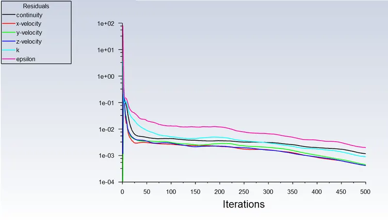
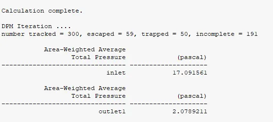
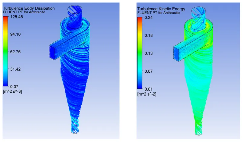
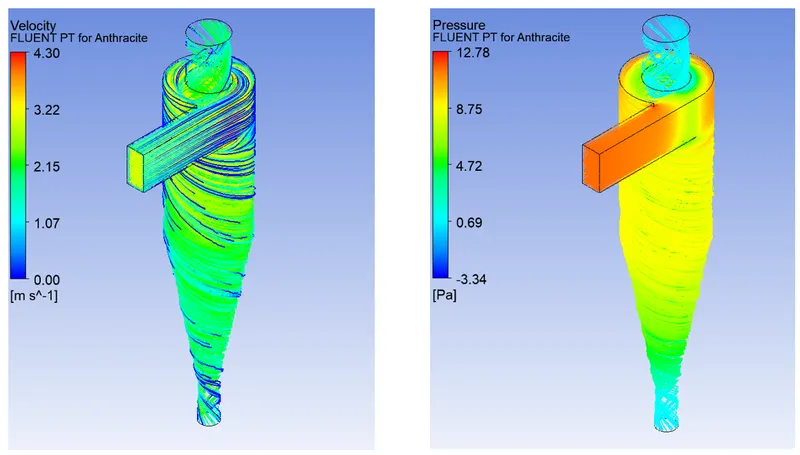
In this simulation the only changes have been made in the injection of particle where the diameter of particle is changed from 1micrometer to 2micrometer. The rest of the simulation setting has been kept constant and another changes is made in the number of iteration which is 500 for this case. The change of iteration size will be discussed in inference section.

1) Residuals

2) DPM Iteration result

3) Turbulent Eddy Dissipation and Turbulent Kinetic Energy

4) Pressure and Velocity

5) Swirling strength and Vorticity

6) Separation efficiency

7) Pressure drop

`∆P=P_i-P_o=17.09-2.07=15.02 Pa`

Result case 3: - (Particle Size = 3µm Velocity = 3m/s)

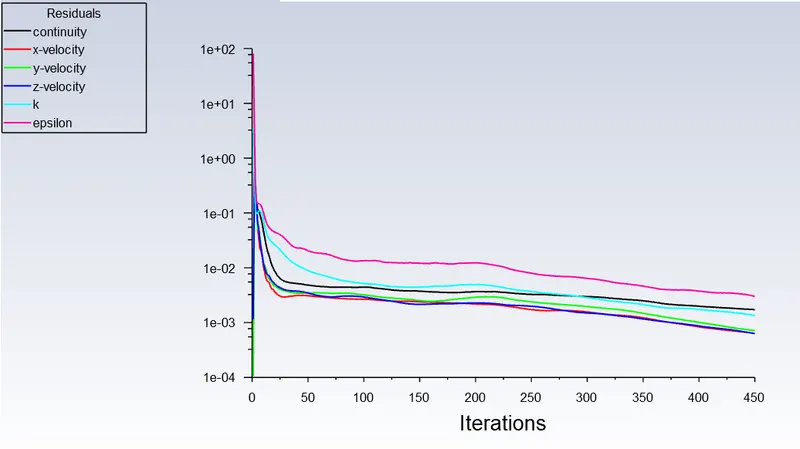
1) Residuals

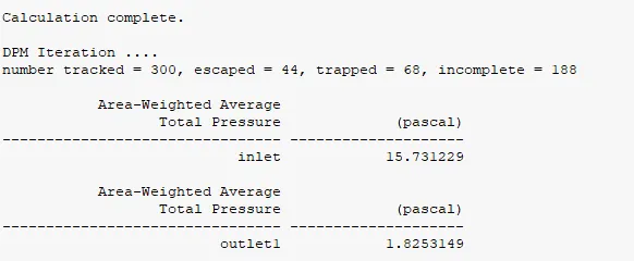
2) DPM Iteration result

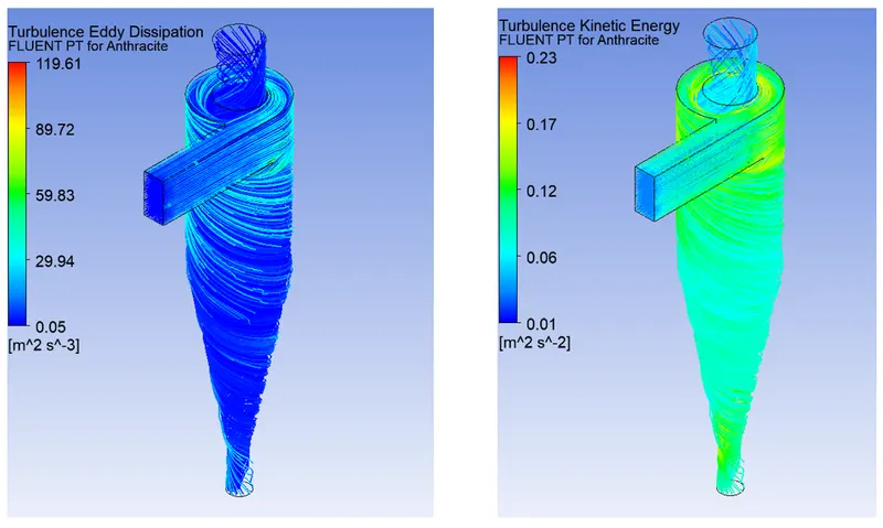
3) Turbulent Eddy Dissipation and Turbulent Kinetic Energy

4) Pressure and velocity

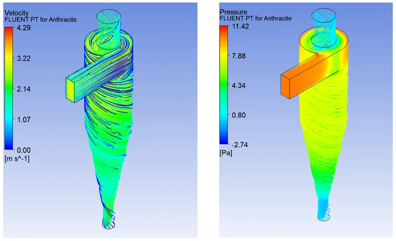
5) Swirling strength and Vorticity

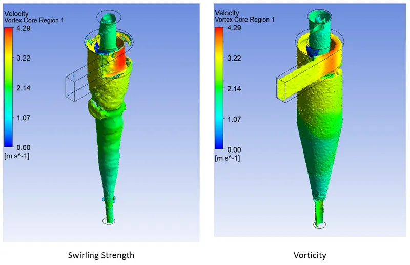
6) Separation efficiency

7) Pressure drop

`∆P=P_i-P_o=15.73-1.82=13.91 Pa`

Result case 4: - (Particle Size = 4µm Velocity = 3m/s)

1) Residuals

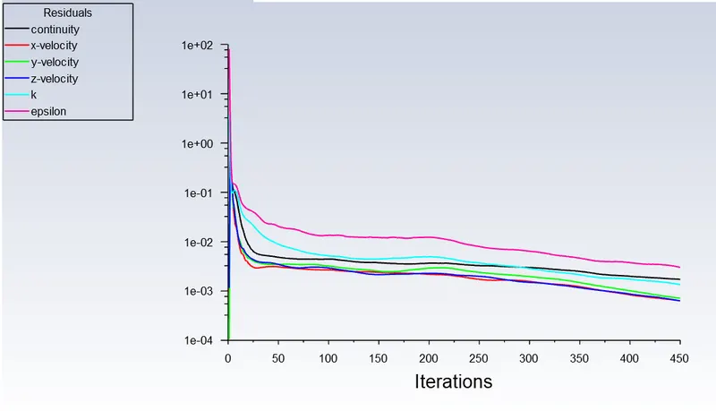
2) DPM Iteration result

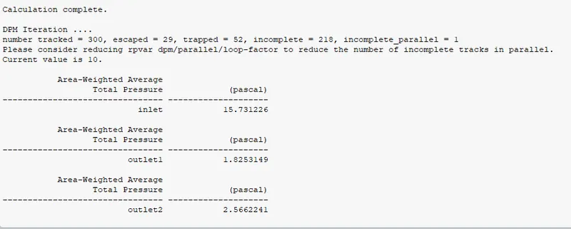
3) Turbulent eddy dissipation and Turbulent Kinetic energy

4) Pressure and Velocity

5) Swirling strength and Vorticity

6) Separation efficiency

7) Pressure drop

`∆P=P_i-P_o=15.73-1.82=13.91 Pa`

Result case 5: - (Particle Size = 5µm Velocity = 3m/s)

1) Residuals

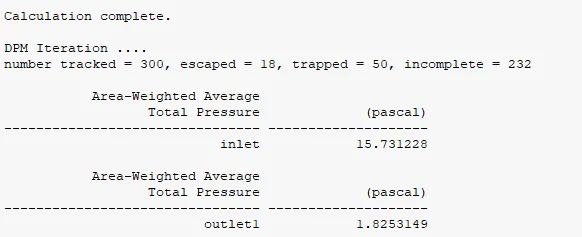
2) DPM Iteration result

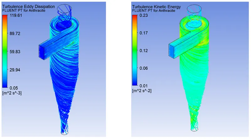
3) Turbulent eddy dissipation and Turbulent kinetic energy

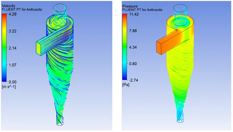
4) Pressure and Velocity

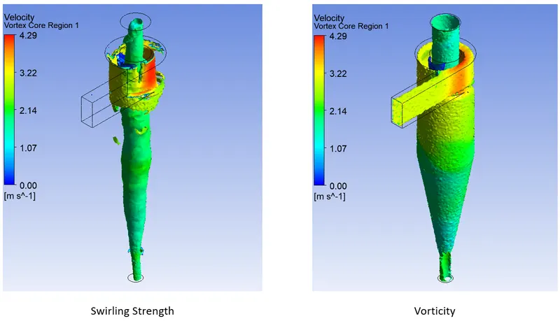
5) Swirling strength and Vorticity

6) Separation efficiency

7) Pressure Drop

`∆P=P_i-P_o=15.73-1.82=13.91 Pa`

Result Table Part 1

Parameters	Particle Tracked	Particle Trapped	Particle Incomplete	Inlet Pressure	Outlet Pressure	Separation efficiency	Pressure Drop
Case 1	300	78	156	8.79	1.67	26%	7.12
Case 2	300	50	191	17.09	2.07	16.67%	15.02
Case 3	300	68	188	15.73	1.82	22.66%	13.91
Case 4	300	52	218	15.73	1.82	17.33%	13.91
Case 5	300	50	232	15.73	1.82	16.67%	13.91

Part 2:

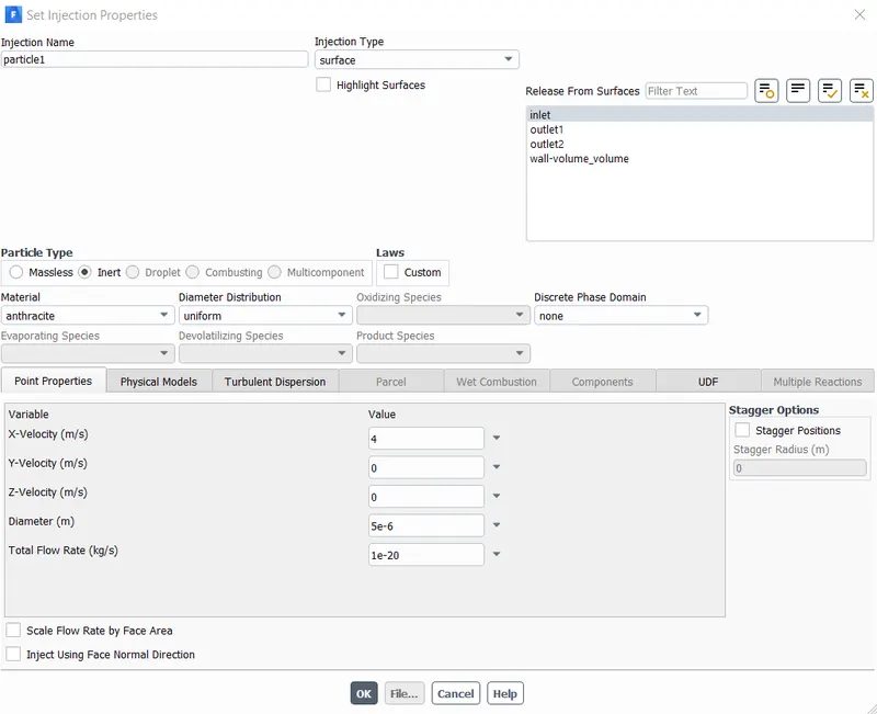
The second part consist of changing the velocity of particle keeping particle diameter as constant. The particle diameter has been kept constant with value of 5micrometer. The velocity is changed from 1 m/s to 5 m/s for each case. The injection paramter are showing below:

The inlet velocity for case number 9 is given as reference which is shown below:

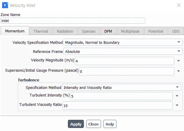
It is advisable to maintain the both inlet velocity as constant for the smooth interaction between the both phase. The results for the all cases are describe below:

Result case 6: - (Particle Size = 5µm Velocity = 1m/s)

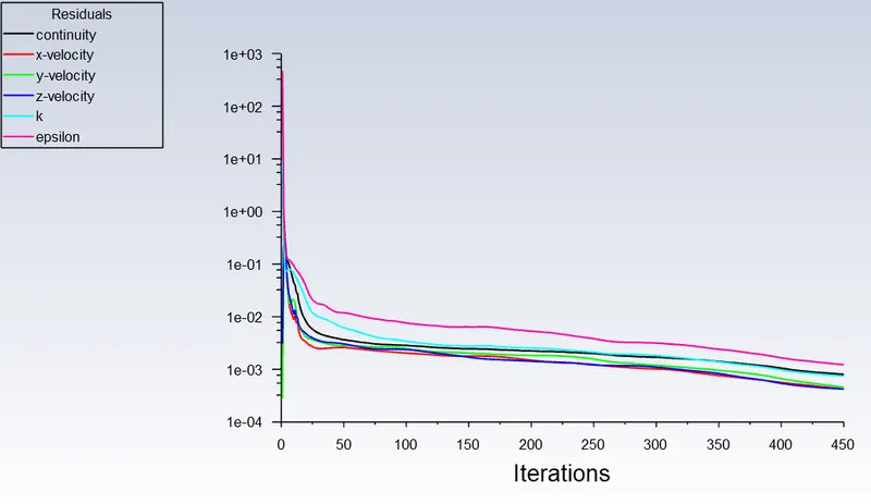
1) Residuals

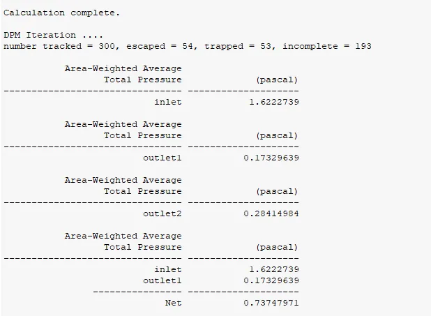
2) DPM Iteration result

3) Turbulent eddy dissipation and turbulent kinetic energy

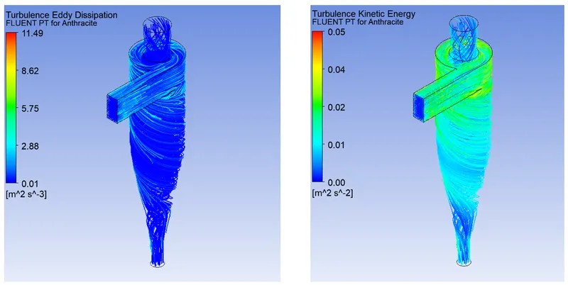
4) Pressure and Velocity

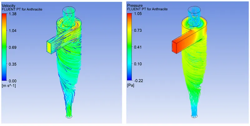
5) Swirling strength and Vorticity

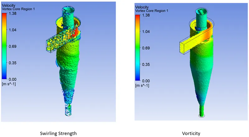
6) Separation efficiency

7) Pressure drop

`∆P=P_i-P_o=1.62-0.17=1.45 Pa`

Result case 7: - (Particle Size = 5µm Velocity = 2m/s)

1) Residuals

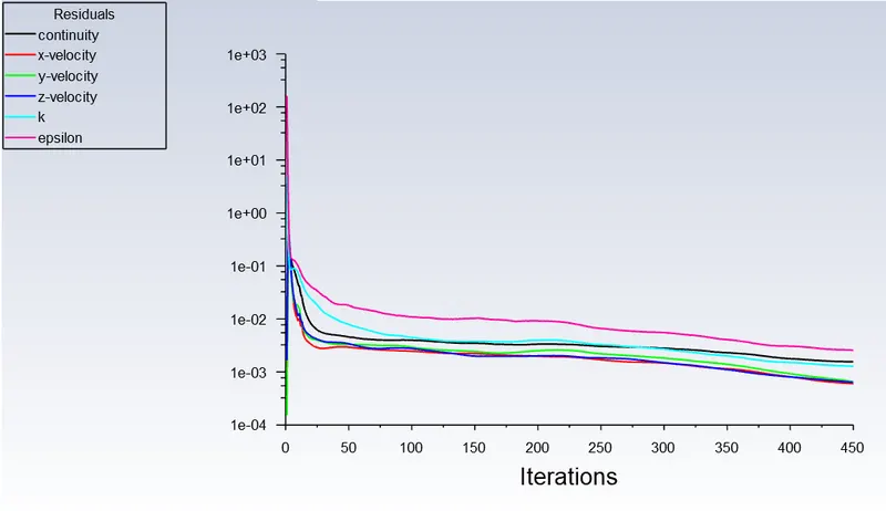
2) DPM Iteration results

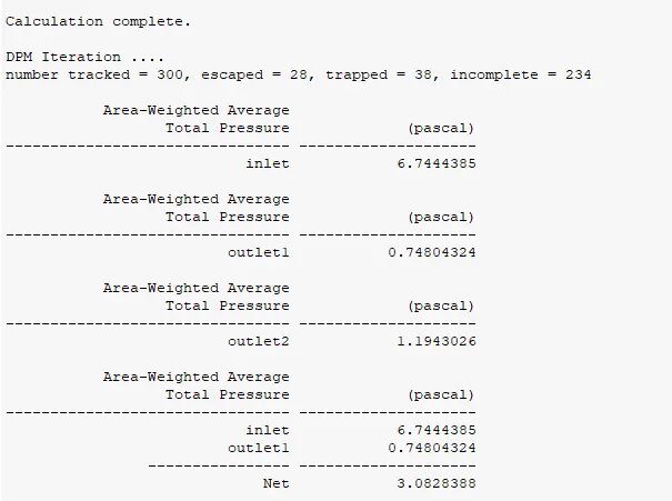
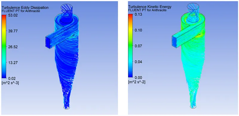
3) Turbulent eddy dissipation and Turbulent kinetic energy

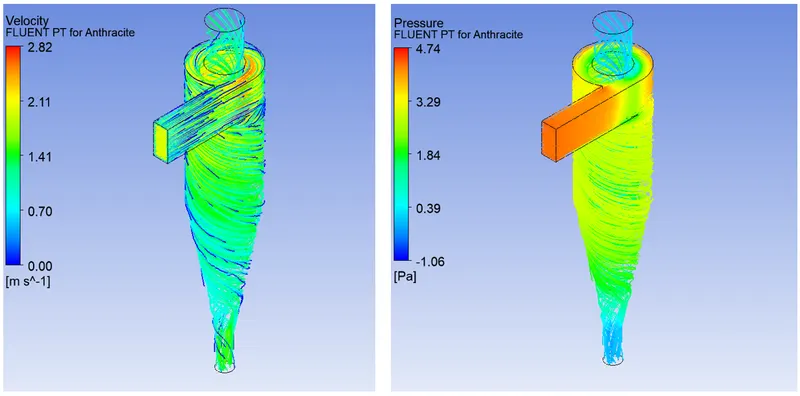
4) Pressure and Velocity

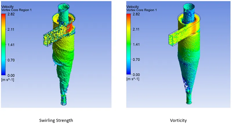
5) Swirling strength and Vorticity

6) Separation efficiency

7) Pressure drop

`∆P=P_i-P_o=6.74-0.78=5.96 Pa`

Result case 8: - (Particle Size = 5µm Velocity = 3m/s)

1) Residuals

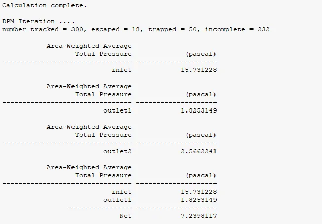
2) DPM Iteration results

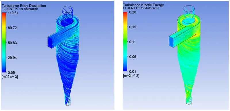
3) Turbulent Eddy Dissipation and Turbulent Kinetic energy

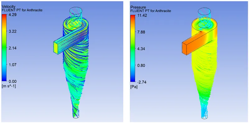
4) Pressure and Velocity

5) Swirling strength and Vorticity

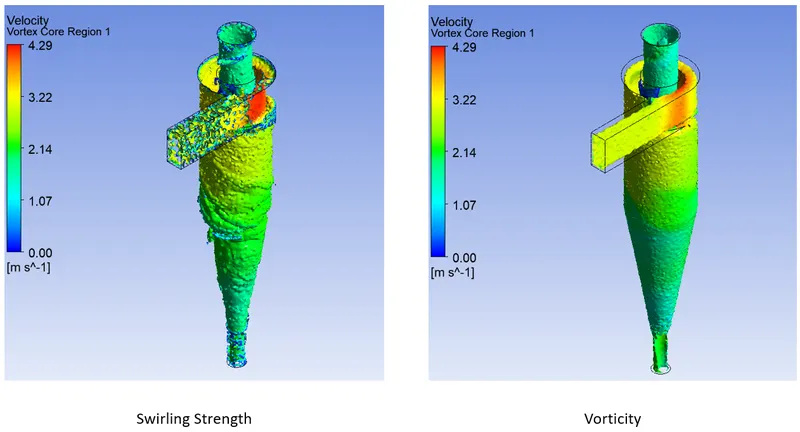
6) Separation efficiency

7) Pressure drop

`∆P=P_i-P_o=15.73-1.82=13.91 Pa`

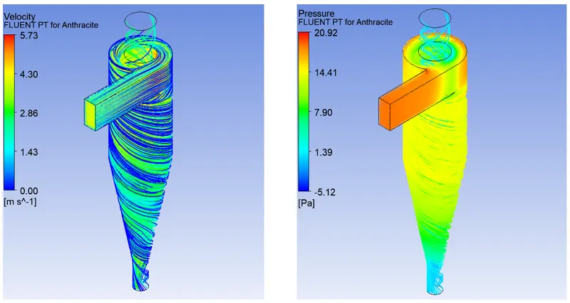
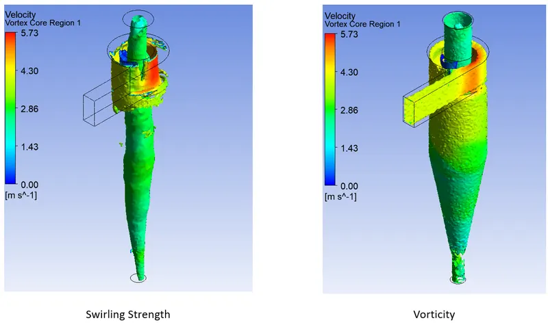
Result case 9: - (Particle Size = 5µm Velocity = 4m/s)

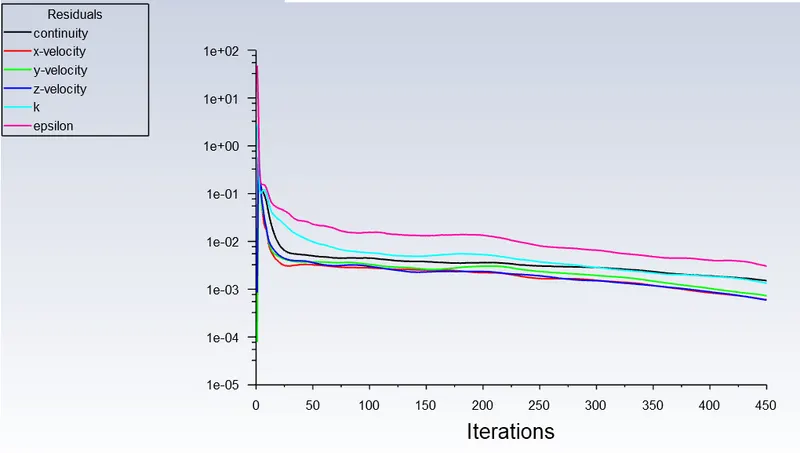
1) Residuals

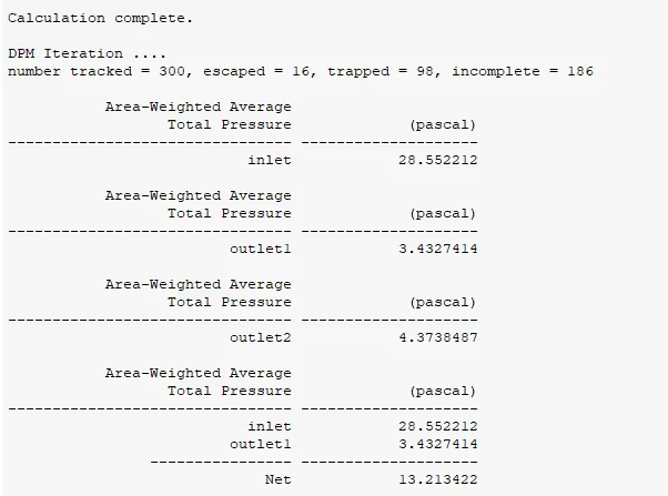
2) DPM Iteration results

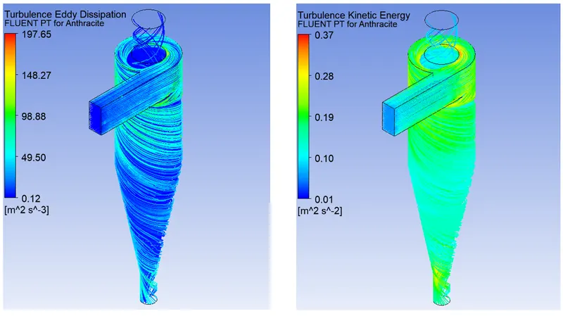
3) Turbulent eddy dissipation and Turbulent kinetic energy

4) Pressure and Velocity

5) Swirling strength and Vorticity

6) Separation efficiency

7) Pressure drop

`∆P=P_i-P_o=28.55-3.43=25.12 Pa`

Result case 10: - (Particle Size = 5µm Velocity = 5m/s)

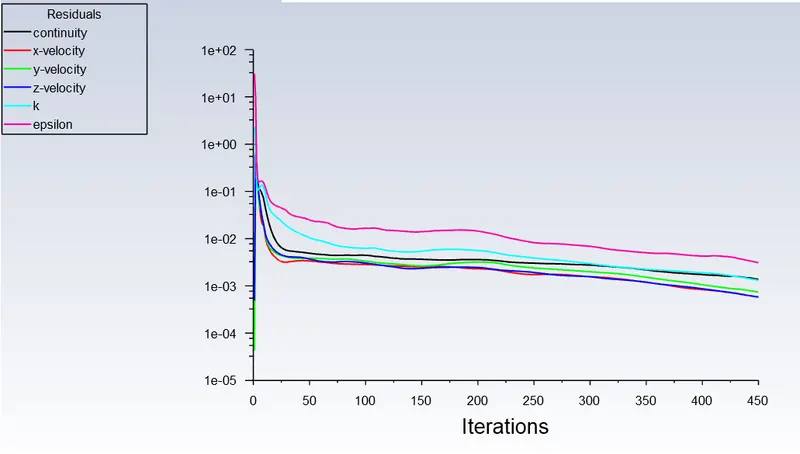
1) Residuals

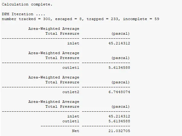
2) DPM Iteration results

3) Turbulent eddy dissipation and Turbulent kinetic energy

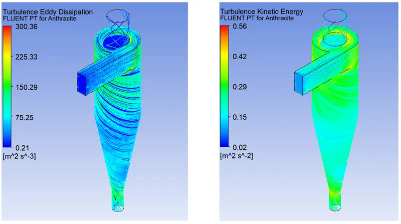
4) Pressure and Velocity

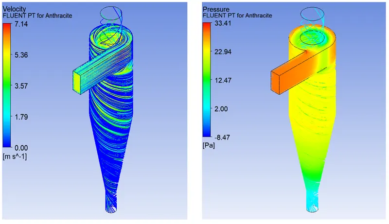
5) Swirling strength and Vorticity

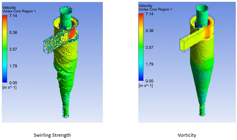
6) Separation efficiency

7) Pressure drop

`∆P=P_i-P_o=45.21-5.61=39.6 Pa`

Result Table Part 2

Parameters	Particle Tracked	Particle Trapped	Particle Incomplete	Inlet Pressure	Outlet Pressure	Separation efficiency	Pressure Drop
Case 6	300	53	193	1.62	0.17	17.67%	1.45
Case 7	300	38	234	6.74	0.78	12.67%	5.96
Case 8	300	50	232	15.73	1.82	16.67%	13.91
Case 9	300	98	186	28.55	3.43	32.67%	25.12
Case 10	300	233	59	45.12	5.61	77.67%	39.6

Conclusion

1) From the simulation of part 1 it can be seen that for first case simulation the efficiency is higher and for the rest of cases it was increasing and decreasing. As per the theory of cyclone separator increase in the particle diameter will eventually increase in the weight of particle which effect the inertia to increase hence more particle has to be settled in the hopper. But in case part 1 simulation the efficiency is lower for other cases. This is cause by the iteration required for DPM calculation and maximum number of steps for tracking parameters.

2) In case of part 2 the same effect is shown for first three cases where the increase in velocity has been provided, but the efficiency is lowered. In case of case 9 and 10 we can see the increase in efficency by twice in size. This is happend because of maximum pressure drop parameter in simulation. Increase in pressure difference cause the particle to move at higher speed hence the tracking parameter for such case predict tracked particle at their best case scenario. Hence it provide better efficiency at the end.

3) From the both case it was evident that the updatation DPM source for every flow iteration should be depend upon the flow velocity and pressure difference of the simulation. Also maximum number of steps should be lowerd as it will put more computational effort on the resources while simulating the problem.

4) The best result for case 1 can be achived by lowering the DPM source iteration in between 2-5. Similarly, number iteration required for calculation of such problem is very essential and this can be done by trial and error method. As number iteration to predict the flow of particle has been converge or not is can't be decided. The convergence for both part of simulation is achived at 679 iteartion. But at the end of iteration the DPM results are very not conviencing as it looks. The number of particle trapped for converge iteration is just 2 out of 300, this make separation efficiency very low.

5) The final result of the DPM particle tracking is mostly depend upon the level of mesh used for the problem. The quality of mesh size of mesh at the specified location of geometry where flow is dominated has to be in better condition so that it can be tracked very easily by solver.