Week 4 - CHT Analysis on Exhaust port
Conjugate Heat Transfer
Aim: Simulation of exhaust manifold with conjugate heat transfer model in ANSYS FLUENT.
Objective: -
- To understand what is conjugate heat transfer.
- To understand how heat transfer coefficient is calculated for internal flow.
- To study effect of Reynolds number on the heat transfer coefficients.
- To prepare geometry for internal flow problem with CHT.
- To setup convective heat boundary condition for simulation.
- To post process the results from simulation and validate with arithmetic equations.
Introduction: -
Fluid flow governs many aspects of natural phenomenon which also includes heat transfer. We know that friction causes to generate the heat within material, at atomic level the molecules start to bounce here and there cause to gain momentum and energy. Similarly, in fluid flow also if viscous fluid is moving around the object it generate heat and transfer heat to outside to gain the equilibrium position. This transfer of heat is one of the basic physics aspect we come across in our normal day to day life. But the question always arise how does this heat get transferred?
We know about mode of heat transfer i.e. conduction, convection and radiation. Conduction is transfer of heat within body, convection is transfer of heat due to air as a medium to atmosphere and radiation is transfer of heat through vacuum which our earth receives from sun every moment. Transfer of heat is nothing but gaining and losing momentum particle when they strike other. In fluid flow when this transfer of heat from fluid to solid happens we called it conjugate heat transfer simulation. Conjugate heat transfer between fluid and solid is always happen at the interface of two, heat transfer rate or coefficient of heat transfer is depending on the Newton’s law of cooling which is given by:
`Q=hA(T_1-T_2 )`
Where,
Q is the heat flux (W)
h is heat transfer coefficient (W/m^2K)
A is the surface area where heat transfer takes place (m^2)
T1 and T2 are the temperature of two objects(K)
From the formulation we can calculate what is heat transfer coefficient which tell us that it is inversely proportional to temperature difference but it is still in non-linear conditions. The application of conjugate heat transfer is varying according to domain. The most important application of this simulations are heat exchangers. In heat exchanger it is important to lower the temperature of working fluid to get desired result, also its main focus on to lower design material from which fluid is flowing. In automobile sector radiator is main heat exchanger to lower the fluid temperature which is supplied to car HVAC system. It uses fins for convection heat transfer between solid and fluid.
Conjugate heat transfer simulation are also used in aerospace industry to design suitable material for engine cover. As the temperature generated during the ignition is high enough to melt certain part of engine cover, hence it is important to know how much this heat transferred to solid part so as to keep parts at rated condition throughout the journey. CHT analysis are also used in the nuclear domain to calculate the heat transfer rate while cooling of nuclear tubes as they generate enormous amount of heat during switch on period. CHT analysis are also used in conjunction with FSI which is fluid structure interaction to determine thermal stresses and deformation of material. The most common application of CHT analysis is HVAC system in which performance of HVAC system is calculated in how much heat is transferred to atmosphere while in working conditions.
Nowadays, CHT analysis are also done in the metallurgical analysis and electronic simulations to determine the heat transferred and acquire by the transistor and capacitors. It is also used to design heat sink. It has also gain importance in simulation of headlights and tail-lights of vehicle. CHT analysis is used in conjunction with DO-radiation model to determine both transfer of heat phenomenon within reflector and bulb or LEDs.
Simulation Methodology: -
The main aspect of this simulation is to calculate the wall heat transfer coefficient by using numerical method and arithmetic method. Also we need know how other factor responsible for heat transfer. The simulation will be perform using three cases in which three different velocities will be used with same temperature range for inlet and outlets.
Case 1: - Inlet velocity 5m/s with inlet temperature 700K.
Case 2: - Inlet velocity 7.5m/s with inlet temperature 700K
Case 3: - Inlet velocity 10m/s with inlet temperature 700K.
For each change in velocity we will calculate the wall heat transfer coefficient and Reynolds number. For all three case the determination of Y plus value is need to be done. As it required for calculation of reference temperature in the simulation.
Calculation of HTC: -
The calculation of heat transfer coefficient is varying from types of flow to how heat transfer takes place. Calculation of heat transfer coefficient is important in the convection flow because it will provide the value due to which amount of heat is transferred to the atmosphere due to air motion. Calculation of heat transfer coefficient is depending upon thermal properties of medium, hydrodynamic characteristic of the flow field and hydrodynamic and thermal boundary conditions. For each mode of transfer there is provision of dimensionless number which can be used to calculate the heat transfer coefficients. Similarly, there is another method to calculate the heat transfer coefficient but by using cell centroid methods.
For convective heat transfer calculations if we consider newton’s law of cooling, the common variables which are used are Twall and Tref instead of T1 and T2 notations. As there is flow field is divided in internal and external flows. In case of external flow, the wall temperature is given by user input as the flow field temperature, but it is necessary to determine the reference temperature. For external flow we can consider far stream flow temperature as reference temperature as shown in figure:
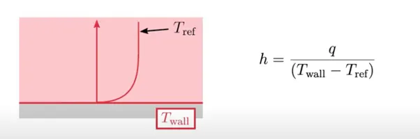
But in case of internal flow the things get complicated and reference temperature is depending upon the mass-flow average temperature which is given as:
`T_(ref)=1/m ̇ ∬(ρ U T dA)`
For cell centroid method the calculation of reference temperature is calculated using Y plus method. In which temperature is consider as function of Y plus value. To calculate the T plus value the equation is given as:
`T^+=(((T_(Wall)-T_(cell) ) ρ C_p C_μ^(1/4) k^0.5 ))/(q )`
We know that relation between heat transfer coefficient and cell temperature as reference temperature which is given as:
`h=q/(T_(Wall)-T_(Cell) )`
`∴h=((ρ C_p C_μ^(1/4) k^0.5 ))/T^+`
As we earlier said about T plus as the function of Y plus value, it is important to determine and calculate the Y plus value for flow domain. The turbulence model also determine what will be the Y plus value for simulation. Using K-ɛ model for the simulation because of two equation model to determine eddy viscosity, the amount of Y plus should be more than 11.25. Considering this mode of turbulence is also good for low Reynolds number flow through pipes. But use of Y plus value to determine the reference temperature to calculate the heat transfer coefficient is more difficult as it will increase the cell count number in simulation. In most of CFD codes like CFX and FLUENT if user know what is the reference temperature near wall then he can directly provide in the software. In CFX it is done using bulk temperature specification and in FLUENT it is provided as reference value.
We have seen how CFD code try to calculate the heat transfer coefficient value in software but it is important to know whether this value which has been calculated from numerical simulation is correct or not. To know how it can be calculated we need to study first turbulence flow in tubes. As the exhaust manifold is the connection of tube it is important to consider this approach. We know that when Reynolds number is less than 2300 we consider it as laminar flow in the tubes. The Reynolds number formula is given as:
`Re=(ρ V D)/μ`
Where,
ρ is density of fluid
V is fluid velocity
µ is dynamic viscosity of fluid
and D is diameter of tube which can be replaced by L if Reynolds number calculate for flat plate.
What we are considering in this simulation is that flow is incompressible with constant properties and fully develop region of a straight circular pipe. It is important to consider the velocity profile as complete in the tube because of characteristic length ‘l’ which can be further determine by L/D ratio. The flow in smooth pipe is fully turbulent for Reynolds number greater than 10000. Most of the time turbulent flow are utilized in the pipe flow because of higher heat transfer coefficients. Most of the correlations of friction and heat transfer are in turbulent flows are based on the experimentation approach because theoretically turbulent flows are difficult to relate.
The heat transfer coefficient can be calculating by assuming friction factor or directly assuming tube is smooth. For smooth tube the friction factor in turbulent flow can be calculated by Petukhov equation which is given as:
`f=(0.790 In Re-1.64)^(-2)` for 10^4 < Re <10^6
By using above equation to determine the friction factor for turbulent flow, the Nusselt number in turbulent flow is given by Chilton-Colburn equation which is given as:
`Nu=0.125*f*Re*(Pr)^(1/3)`
For fully developed turbulent flow in smooth tubes, a simple relation for the Nusselt number is obtained by providing simple substitution of power law for friction factor which is given as:
`f=0.184Re^(-0.2)`
If above equation is put in previous Nusselt number equation, it will provide well governed equation of Dittus-Boelter which is given by:
`Nu=0.023 Re^0.8 (Pr)^n`
This equation is applicable if 0.7<Pr<160 and Re>10000
From the Nusselt number we can calculate the heat transfer coefficient as:
`Nu=h/(k/l)`
Where,
h is heat transfer coefficient
k is the thermal conductivity of fluid
and l is characteristic length.
As we have got all the equation for calculating heat transfer coefficient we can now extract the same for our case. The given data for air as a fluid, the properties of air given as:
- Density of Air = 1.225 Kg/M3
- Dynamic Viscosity = 1.7965E-5 Kg/m.s
- Specific heat = 1.006E+3 J/kgK
- Thermal Conductivity = 0.0252 W/mK
- Prandtl number = 0.7165
- Diameter of Pipe = 0.17 m
- Velocity of Air = 5 m/s
A) Calculation of Reynolds Number
`Re=((ρ*V*D))/μ=((1.225*5*0.17))/(1.7965E-5)= 57959.922`
As we can see the calculated value for Reynolds number is more than 10000 hence the flow is turbulent in nature.
B) Calculation of Nusselt Number
`Nu=0.023 Re^0.8 (Pr)^n`
`Nu=0.023*(57959.922)^0.8*(0.7165)^0.3`
`Nu=134.522`
C) Calculation of Heat Transfer Coefficient
`Nu=h/(k/l)`
`h=Nu*k/l=134.522*(0.0252/0.17)=19.94 W/m^2 K`
The above calculation is done in respect without consideration of friction factor in the simulation. The calculation which is done is not much accurate, it is evident that considering friction factor will improve the solution also increase the heat transfer coefficient. The calculation of heat transfer coefficient with Dittus-Boelter equation provide almost 25 percent of error which need to be minimize by second Petukhov equation which is given as:
`Nu=(((f/8) (Re-1000)*Pr))/(1.07+12.7*(f/8)^0.5*((Pr)^(2/3 )-1) )`
The validation of above equation is in range of for 0.5<Pr<2000 and 104 <Re< 5 x 10⁶
For the calculation of heat transfer coefficient for above equation it is important to know about roughness of tube. The roughness can be calculated by using Colebrook equation which is depend on Reynolds number and relative roughness ɛ/D.
`1/(√(f ))= -2.0 log(((ε/D))/3.7+2.51/(Re* √f))`
If we can associate value with respect to friction factor equation our f will be 0.0312 and if this value put in second Petukhov equation to calculate the Nusselt number, we will get 192.63 and the resultant heat transfer coefficient is 28.55 W/m2K.
Hence from the calculation we can notice that providing friction factor in calculation of heat transfer coefficient will greatly affect the value at higher side which means more heat transfer through the pipe to the atmosphere. In real life manufacturing we consider the roughness as no surface is 100% smooth. Beside of that calculation of heat transfer coefficient with second Petukhov equation gives only 10% error rather than Dittus-Boelter equation.
Solving & Modelling: -
Solution methodology is being discussed earlier in which this simulation will be done in three cases with increase in velocity. The simulation will start from pre-processing of the geometry in which we are going to use space-claim pre-processor to make model ready for simulation. After geometric modelling it is important to create the mesh and check the quality accordingly. First we will create a baseline mesh for case 1 and similarly refine the mesh parameters. The calculation of Y plus is done according to turbulence model we are using for simulation.
Now it is important to consider what is desired result from the simulation, because it will change the aspect view toward the problem. In our problem we are more interested in calculating heat transfer coefficient on the wall of solid i.e. how much is heat is transferred from fluid to solid. As the flow is turbulent in nature, the near wall treatment is valuable and preferred in most of the cases. If we want to capture viscous layer of turbulent flow gradient then it is necessary to provide lower Y plus value for simulation, and if we are interested in capturing viscous layer and buffer layer of turbulent flow then Y plus value should be near to 50. From some literature it is determined that when the flow is fully turbulent the heat transfer from the boundary layer is maximum. As we have known that boundary layer thickness is essential for the problem with Y+ value ranging 30-50, now we need to select what turbulence model is need to be use.
For turbulence model associated with energy equation and low Reynolds number should be treated with 2 equation model i.e. K-epsilon or K-omega model. There are more literatures available for choosing either K-epsilon or K-omega models. If we consider the standard K-epsilon model, it is robust turbulence model and used widely despite of limitation of models. But it performs very poorly for complex flows involving pressure gradient, flow separation and strong streamline curvature. So another turbulence model in K-epsilon family is Realizable K-epsilon model which can be treated for boundary layer flows with moderate swirls and vortices and locally transitional flows, but the disadvantage of taking more time converge. The better offer compared with K-epsilon is given by standard K-omega model which is most favorable to use against low Reynolds flow with wall bounded boundary layer.
So as we have discussed the importance of each of turbulence model, we will make some change with in the simulation cases, all the cases will be simulated with realizable K-epsilon model and standard K-omega model with desirable Y plus value of 50 for both turbulence model. The calculation of total thickness of inflation layer is given below:
1 – Calculation of Reynolds Number
`Re=(ρVD)/μ=(1.225*5*0.17)/(1.789e^(-5) ) =57959.922`
2- Calculation of skin friction coefficient
`C_f=0.079/(Re^(1/7) )=0.079/(57959.922)^((1/7) ) =0.01648`
3- Calculation of Shear stress near wall.
`τ_(wall)=(C_f*ρ*U^2)/2=(0.01648*1.225*(5)^2)/2=0.2524 N/m^2`
4- Calculation of Friction velocity
`U_(Fric)= √(τ_(wall)/ρ )= √(((0.2524))/((1.225) ))=0.4538`
5- Calculation of first layer thickness
`ΔS=(Y^+*μ)/(U_(Fric)*ρ) =((50*1.78e^(-5) ))/((0.4538*1.225))=0.003477 m`
6- Total thickness of Inflation for 5 layer
`Total ThickNess=3.4*((1.2)^5 )=8.46 mm`
1. Geometry Modelling
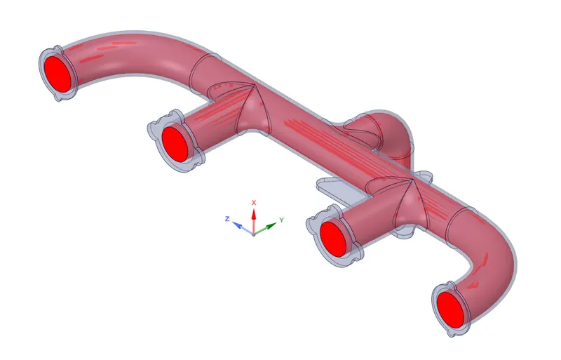
Geometry is imported directly in the space-claim software but before proceeding to simulation directly it is need to be pre-processed. For internal flow simulation with conjugate heat transfer it does require both solid and fluid domain for simulation. To create the fluid domain inside solid geometry volume extract command is used, in which edge extract provide better result to create volume. After extracting the fluid volume, the geometry is shown below:
For conjugate heat transfer it is important to have conformal mesh between solid and fluid domain because of better heat transfer. Non-conformal mesh is also get valid result but it can be used in geometry which are more complex. Complex geometry gives more difficulty for creation of conformal mesh hence it depends on the user to use conformal mesh or non-conformal mesh. In space-claim to have conformal mesh it is necessary to have both geometries share the faces accordingly. This is done by using workbench option in space-claim in which share topology option can be used. After applying the command, the geometry will look like:
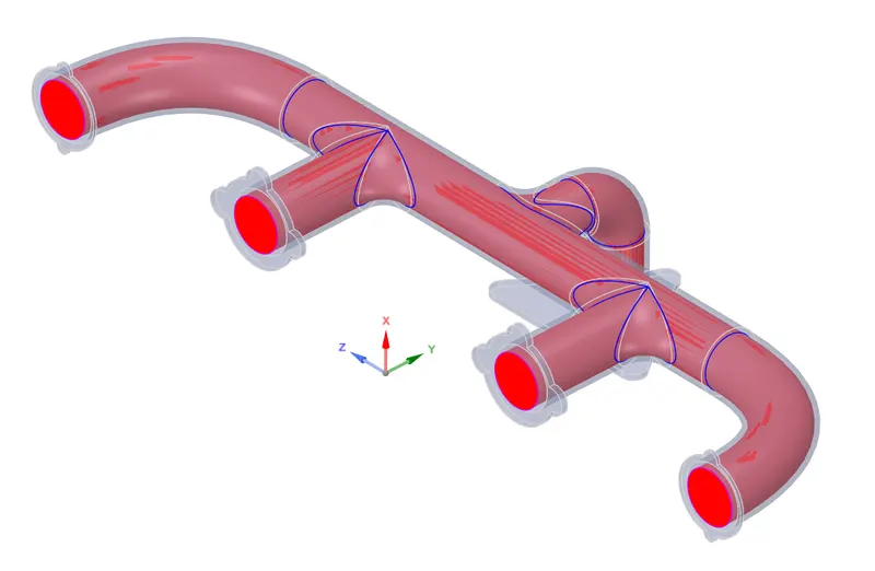
From the above geometry we can see that the blue lines are shared edges between solid geometry and fluid domain.
2. Meshing – Baseline Mesh with K-epsilon Turbulence model
In the first case of meshing we will use baseline mesh for simulation. The baseline mesh will be done using default meshing parameters from workbench applied for FLUENT as mesh physics option. Below figure shows the baseline mesh:
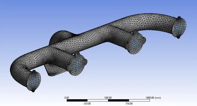
The total amount of element created using baseline mesh are 137832 and the quality criteria are shown below:
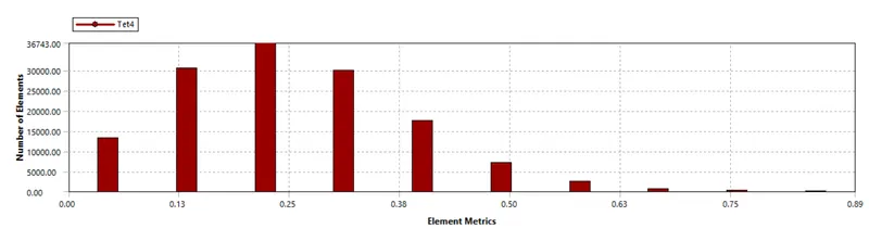
Skewness
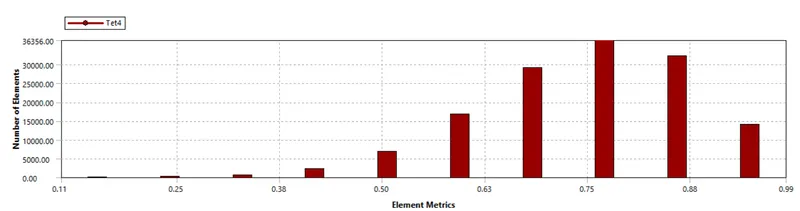
Orthogonal Quality
From the both quality criteria skewness and orthogonal quality, all the element present in the mesh are only tetrahedral elements and with good quality criteria which means we can go further with simulation. Before operating FLUENT for simulation it is necessary to create the named selection for boundary conditions. The named selections are shown as:
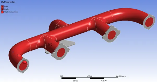
As we can see in above image, the four inlets are provided to the fluid domain and one outlet also, and convection boundary condition is applied to exhaust manifold section.
3. FLUENT Setup
After completing the meshing and setting up named selection for boundary conditions, FLUENT setup is required for completing the simulation. Main aspect to first start in FLUENT is to scale the geometry by default unit system. As we are taking meter as unit to measure all the arithmetic calculation same unit system required in the FLUENT also. After that material has to be created, in FLUENT if there is both solid and liquid domain present, then FLUENT by default provide AIR as material to fluid domain and ALUMINUM to solid domain. We will keep the material by default, the material for air is shown below:
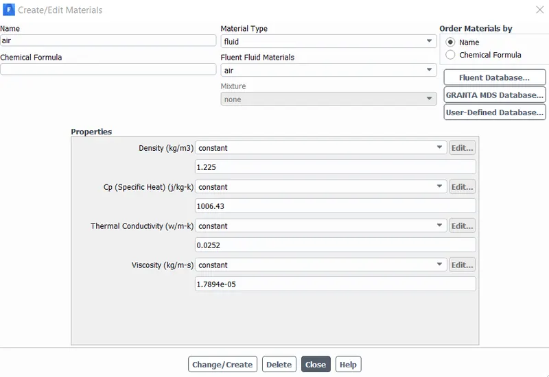
After selecting material for both domains, the need is to select the proper turbulence model. As discussed earlier we will go with K-epsilon with realizable setup and with energy equation is activated for energy equations. The turbulence model setup is shown below:
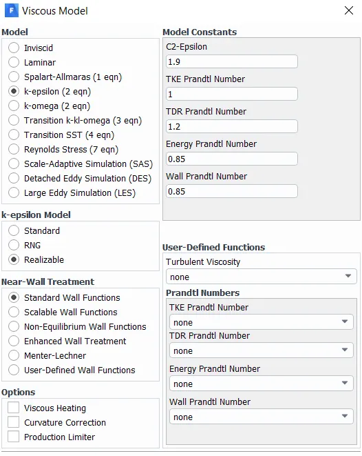
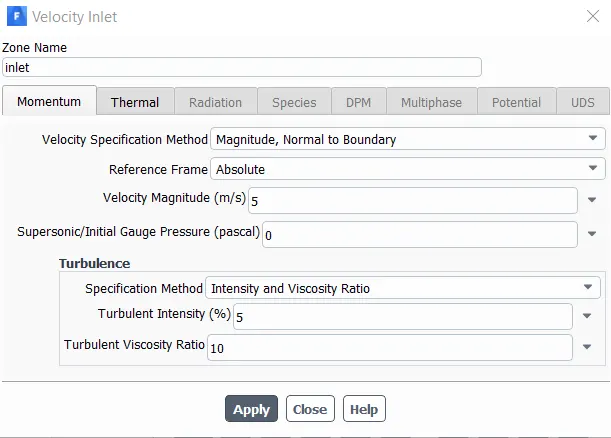
Completing the setup for flow field moving further to provide information about boundary conditions. The inlet boundary condition is velocity inlet with 5m/s velocity and 700K as inlet temperature in exhaust manifold. The inlet boundary condition is shown below:
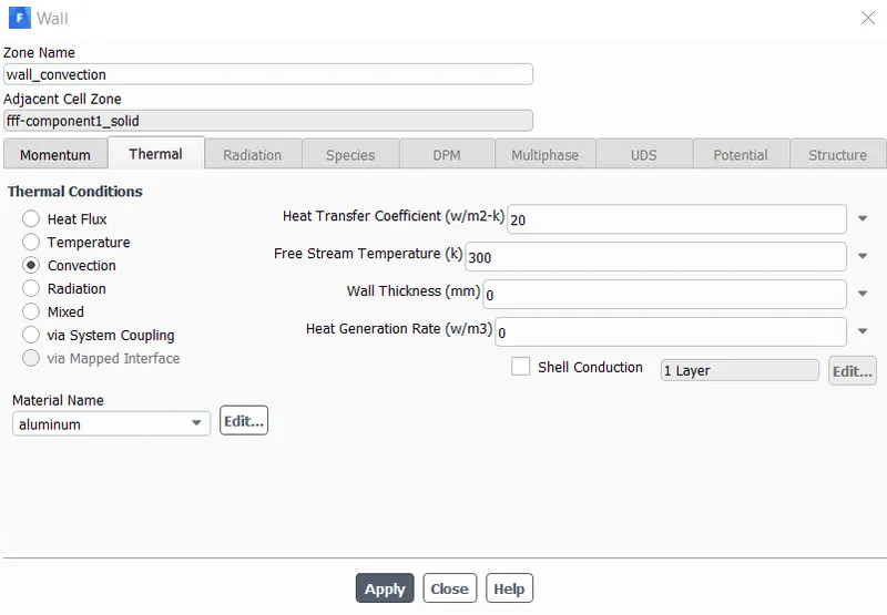
The outlet boundary condition will be pressure outlet with 300 kelvins as outside temperature. The named selection of wall convection is treated as wall boundary condition in FLUENT and thermal boundary condition has to be imposed on it in form of convection boundary condition with heat transfer coefficient of 20 W/m2K. The image of convection boundary condition is shown below:
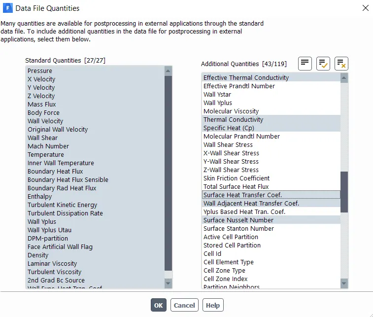
Moving further pressure velocity coupling scheme has to be select for problem which will be consider as SIMPLE for low Reynolds number mostly. There should be some plot about which we can determine whether simulation is converged. This is done by using monitor tool in FLUENT and making wall convection to report temperature data. After initialization the animation of contour of temperature on inlet, outlet and convection wall has to be created for making animation of it. Before solving the problem it’s better practice to create some user defined solution reports which can be done by data file quantities, in which all the output results are present which will be further carried in the post-processing. The main output data files which need to be post-process are wall heat transfer coefficient and surface Nusselt number. The data file quantities are shown below:
The simulation will be run for 700 iterations and animation will be save for interval of 10 iterations to lower the memory database. The results for baseline simulations are given further.
4. Result Baseline Simulation
The result we are much needed attention are residual plot from which we can say that convergence is occurred or not. Similarly, we are looking for temperature plot on the convection wall to know whether temperature reaches its steady state value.
A) Residual plot
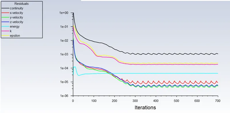
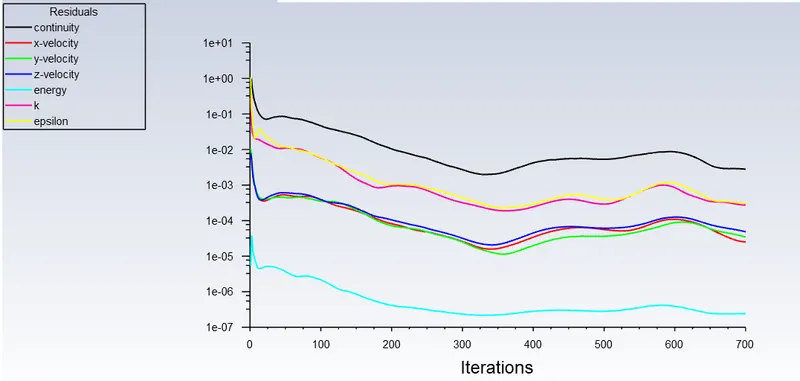
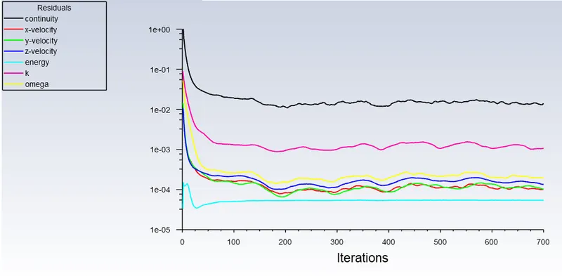
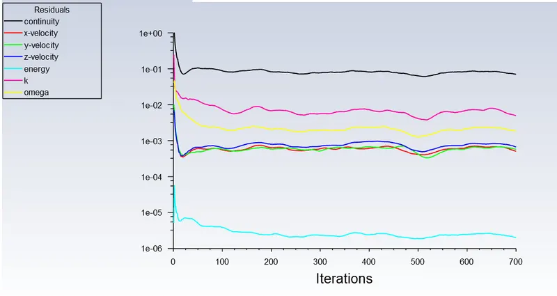
What we can see from residual plot it that results are near to convergence but it requires more iteration. Performing more iterations will take more time, to have better understanding of results we need to have other plot. In this case temperature stabilization is main focus of simulation.
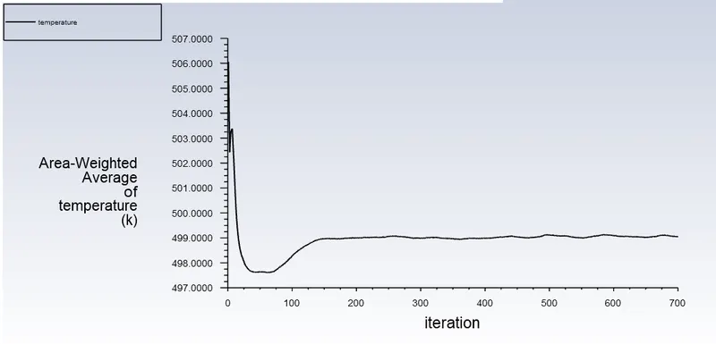
B) Temperature Plot
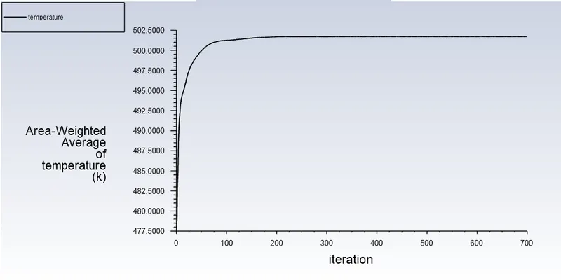
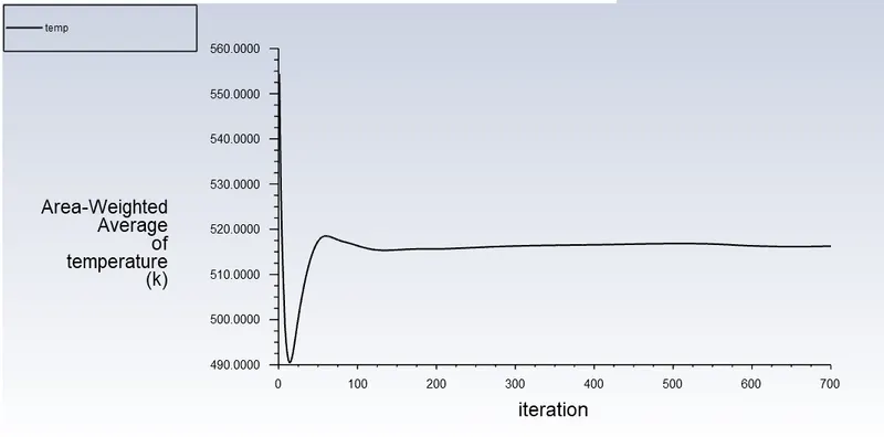
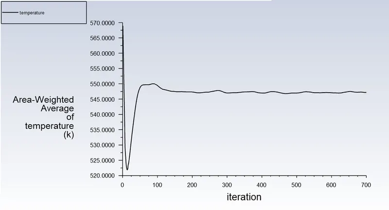
From above plot it is quite confident that temperature is stabilize from 250 iterations and there is only small change in temperature, which we can say that solution is complete for what we required. The simulation time for the problem is 3 minutes and 10 seconds.
C) Temperature Contour on Convection wall
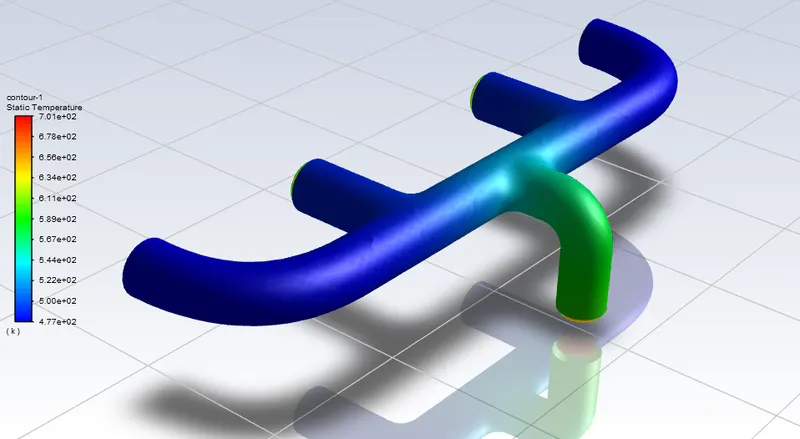
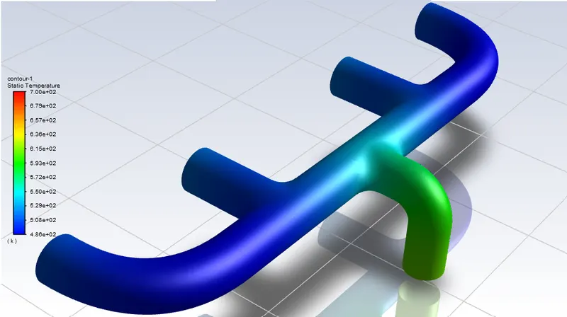
From the above image we can see that, temperature has been stabilize very early iteration and kept constant for almost 350 iterations. We can see temperature distribution very clearly and it is seeming that temperature is higher at where outlet bend has started.
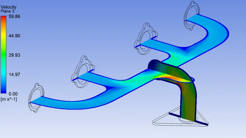
D) Velocity Contour on Cut plane
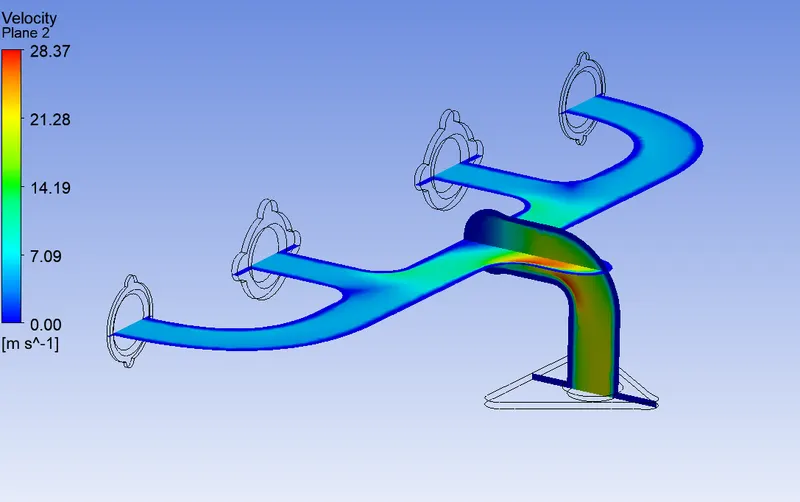
E) Temperature contour on cut plane with streamlines
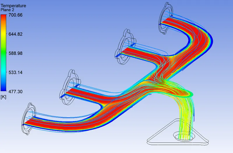
F) Heat transfer coefficient with streamline
G) Velocity and HTC chart
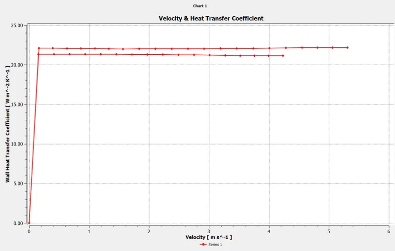
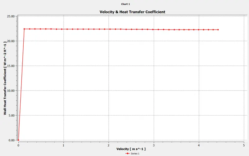
From the above chart we can say that, for the velocity of 5m/s what we have calculated is under the range of heat transfer coefficient from the simulation.
Case 1: - Velocity 5m/s with inflation- Realizable K-epsilon model.
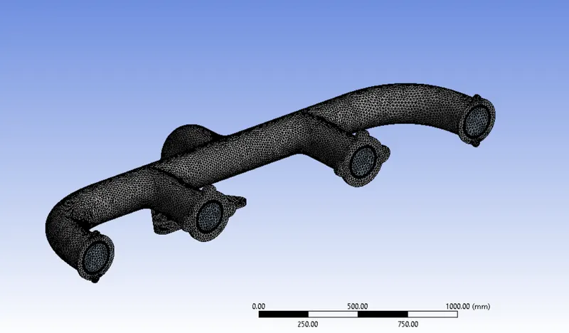
As we can see from baseline mesh simulation the results are quite good but not at par because of mesh refinement. In the first case we are going to use mesh inflation for calculated Y plus value with same turbulence model used for baseline simulation. The mesh of the first case simulation is shown below:
Expanded view of mesh at fluid and solid interface.
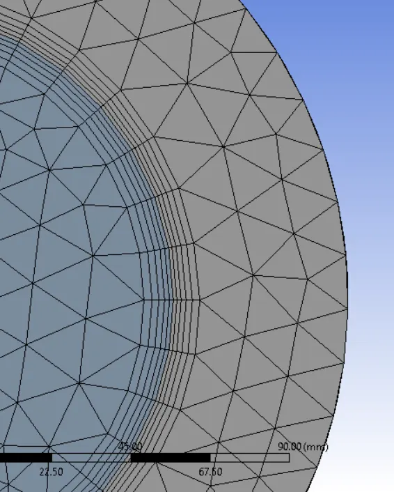
The amount of element created in the mesh setup are 505172. This simulation has been again run for 700 iterations and results were provided accordingly.
Results Case 1: -
A) Residual
B) Temperature plot
C) Temperature contour on convection wall
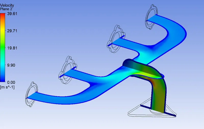
D) Velocity Contour on cut plane
E) Temperature contour on cut plane
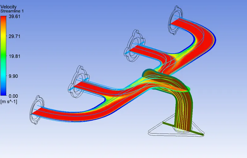
F) Heat transfer coefficient
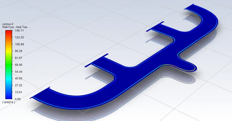
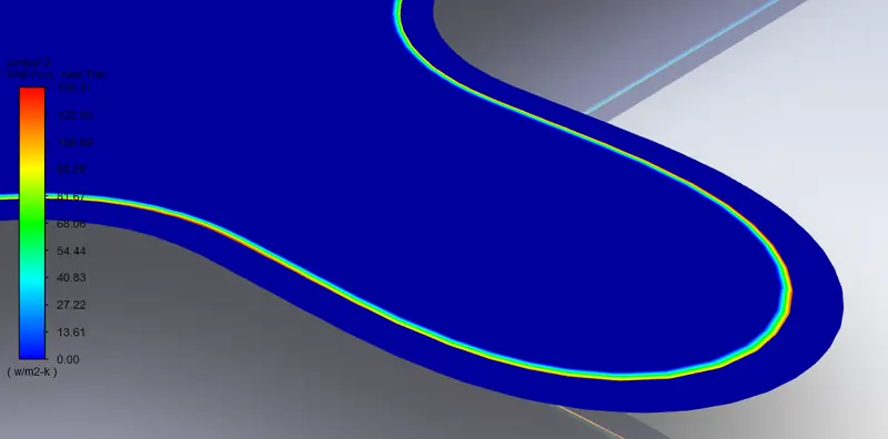
G) Heat transfer coefficient with expanded view
Case 2: - Velocity 7.5m/s with inflation- Realizable K-epsilon model.
In second case all the things will be same despite of increase in velocity from inlets. It is done in respect of providing factors which are affecting wall heat transfer coefficients. The calculation of heat transfer coefficient for the velocity of 7.5m/s is given as:
A) Calculation of Reynolds Number
`Re=((ρ*V*D))/μ=((1.225*7.5*0.17))/(1.7965E-5)= 86939.88`
As we can see the calculated value for Reynolds number is more than 10000 hence the flow is turbulent in nature.
B) Calculation of Nusselt Number
`Nu=0.023 Re^0.8 (Pr)^n`
`Nu=0.023*(86939.88)^0.8*(0.7165)^0.3`
`Nu=186.066`
C) Calculation of Heat Transfer Coefficient
`Nu=h/(k/l)`
`h=Nu*k/l=186.066*(0.0252/0.17)=27.58 W/m^2 K`
The first layer thickness of inflation layer for the mesh parameter is 2.4mm and total thickness is 5.97mm. The mesh after providing inflation is shown below:
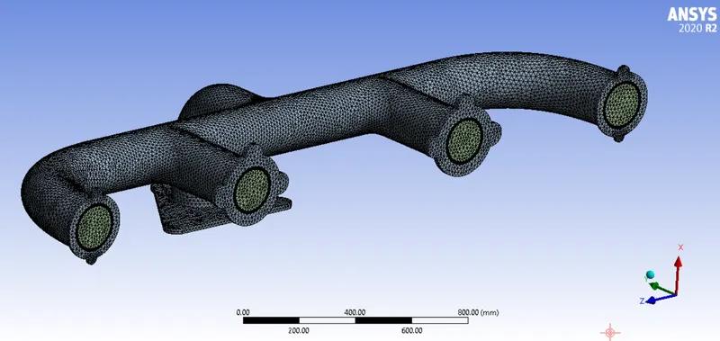
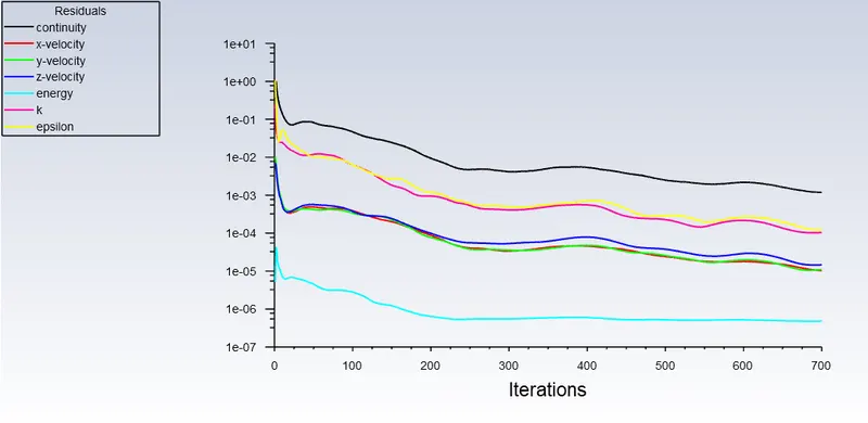
Results Case 2: -
A) Residual
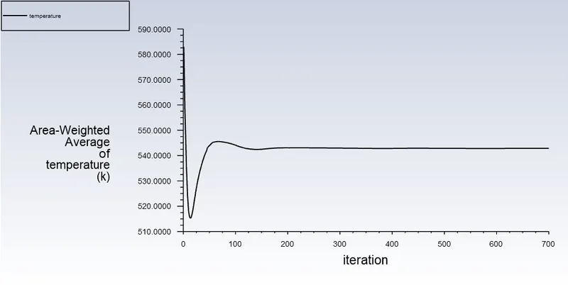
B) Temperature plot
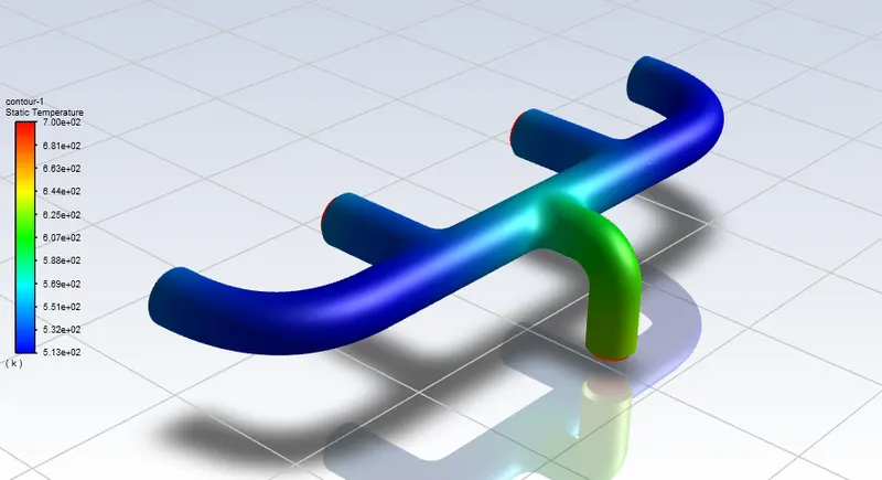
C) Temperature contour on Convection wall
D) Temperature contour on cut plane
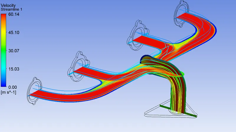
E) Velocity contour on cut plane
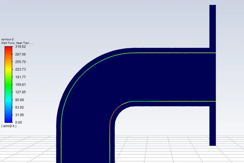
F) Heat transfer coefficient
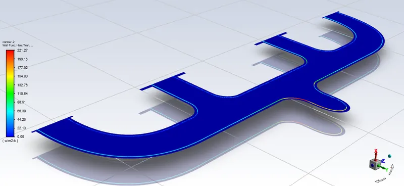
The heat transfer coefficient from CFD simulation is around 28.25 W/m2K. The results are closer to the arithmetic solution and we can see in above image that as velocity is increased the heat transfer coefficient in the area has also increased because of turbulence.
The case 3 & 6 simulations will be directly provided in the Table form, we will move directly to case 4 and 5 simulation in which we are going to use the Standard K-omega model for simulation with inflation layer.
Case 4: - Velocity 5m/s with inflation and Standard K-omega Model
In previous discussion we have seen what is the advantage of K-omega model and how can it treat flow better as compare to K-epsilon model. Keeping rest of things similar to case 1 and running 700 iterations the results are shown below:
Results Case 4: -
A) Residual
B) Temperature plot
C) Temperature contour on convection wall
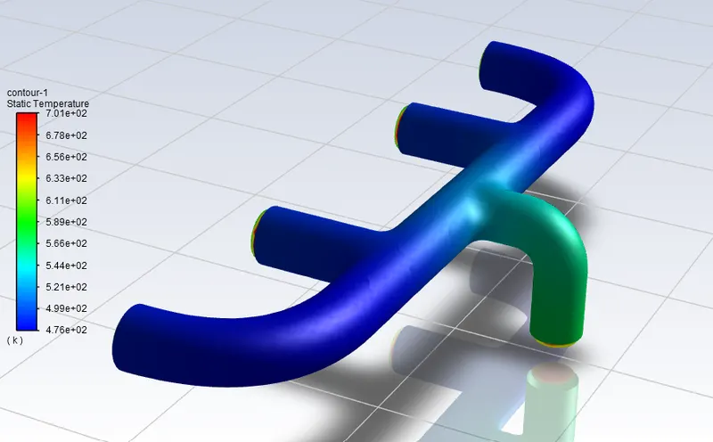
D) Temperature contour on cut plane
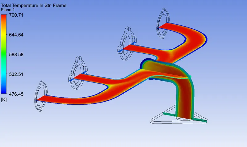
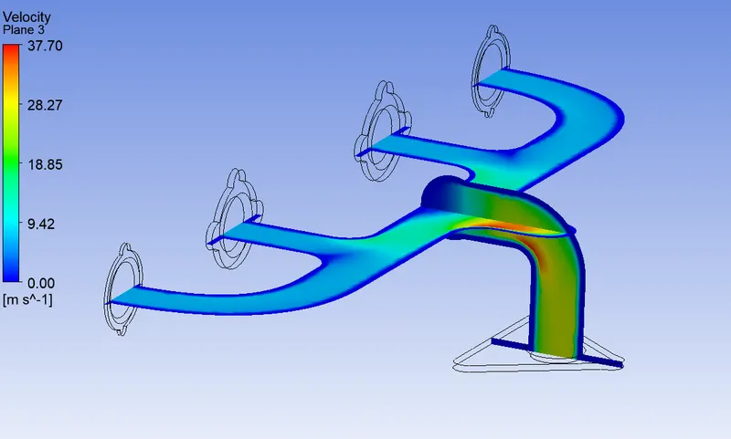
E) Velocity contour on cut plane
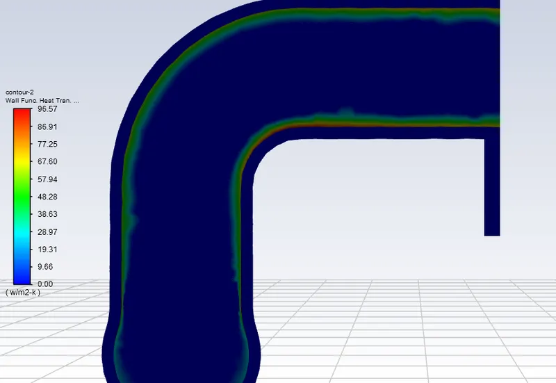
F) Heat transfer coefficient
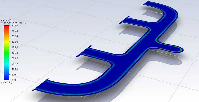
G) Heat transfer coefficient expanded view
H) Velocity and HTC chart
Case 5: - Velocity 7.5m/s with inflation and Standard K-omega Model
Results: -
A) Residuals
B) Temperature plot
C) Temperature contour on convection wall
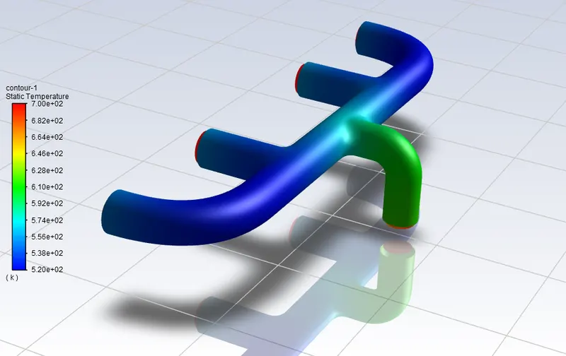
D) Temperature contour on cut plane
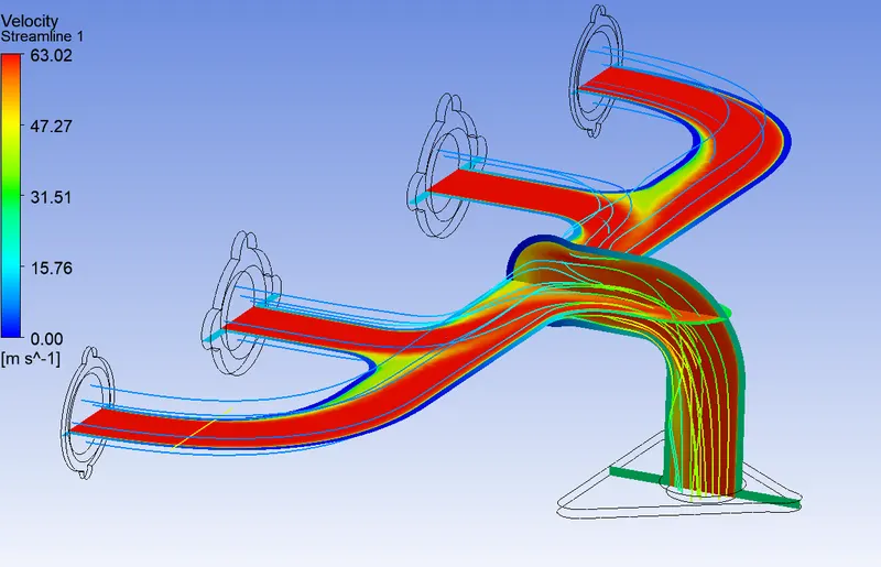
E) Velocity contour on cut plane
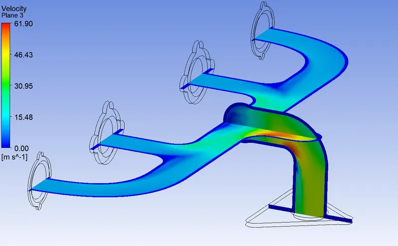
F) Heat transfer coefficient
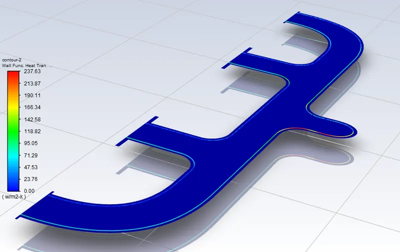
G) Heat transfer coefficient expanded view
Result Table: -
|
Parameters |
Calculated HTC |
Simulated HTC |
% Error |
|
Case 1 |
19.94 |
22.78 |
14.24 |
|
Case 2 |
27.58 |
28.25 |
2.42 |
|
Case 3 |
34.71 |
35.62 |
2.62 |
|
Case 4 |
19.94 |
22.21 |
11.38 |
|
Case 5 |
27.58 |
28.10 |
2.10 |
|
Case 6 |
34.71 |
35.16 |
1.29 |
Conclusion: -
1) From the simulation of exhaust manifold it was evident that the calculated value of heat transfer coefficient are in range of less than 15% error with CFD results. But the simulation has been carried out without considering any friction factor which would have provided better results for cfd simulation.
2) The simulation was carried with two different turbulence model and with different velocities. From the results of residual plot we can say that Relizable K-epsilon model converge faster as compared to Standard K-omega model also later one required more iteration for stabilization. From the average temperature plot on the convection wall it was seen that Relizable K-epsilon model took lower iteration to get stabilize as compared to standard K-omega model. Whereas, from the table we can say that the percent error is lower in Standard K-omega model as compared to Relizable K-epsilon model. In the end it is beneficial to use Relizable K-epsilon model for the simulation as it was providing results faster and with great convergence ratio.
3) In all the cases we found that heat transfer coefficient increasing where value of velocity is greater which shows that increasing in turbulence cause the brownian motion to setup and cause fluid particle near to wall accelerate. Providing inflation layer is one of the best mesh input could be utilize for such simulation as we had seen in the baseline simulation it was very difficult to predict the heat transfer coefficient near the wall but after providing inflation we can get better visualization near the wall boundaries.
4) For the note on accuracy of prediction of heat transfer coefficient is greatly depend on the velocity of flow means reynolds number and nusselt number. If one calculate the arithmatic value heat transfer coefficient and provide similar to simulation then after simulation we can see it matches with calculated value.
References:
1) [CFD] Heat Transfer Coefficient (htc) in ANSYS Fluent, OpenFOAM and CFX - YouTube
2) https://www.youtube.com/watch?v=SVYXNICeNWA
3) HEAT TRANSFER COEFFICIENT (thermopedia.com)
4) Yunus A Cengel "Heat Transfer A Practicle Approach"