Week 5 - Rayleigh Taylor Instability

Rayleigh Taylor Instability

Aim: - Study and Simulation of Rayleigh Taylor Instability using VOF method.

Objective: -

• To study importance of Rayleigh Taylor Instability.
• To study multiphase flow in ANSYS FLUENT.
• To study volume of fluid method and its importance.
• To study effect of mesh refinement on the Rayleigh Taylor instability.
• To study and calculate Atwood number for difference of density simulation.
• To explain behavior of instability based on Atwood number.

Introduction: -

Fluid flows are mostly dominating with single phase in the application toward the pipe flow and other transporting medium. In recent application of industrial development multiphase flows are introduced and gaining more popularity. Multiphase flow is the concept in which two or more different liquids may be immiscible or not are used to complete the task. The multiphase flow can be of two similar liquids with different density or gas-liquid flow depending upon applications. The application of multiphase flows is in chemical industry, nuclear industry, production plants and agitator mixing of different products.

Rayleigh Taylor instability is one of the sector of multiphase flow which is based on the density stratification in which heavier fluid is on top of lighter fluid which is inherently unstable. A small perturbation can be providing to the interface which will allow fluid to displace in the field of gravity. The cause of instability is mostly depending on the density of the two liquids. The governing equation which resembles the Rayleigh Taylor instability in 2 dimension is mostly assumed on the basis of two immiscible liquids i.e. viscosity of liquids is not consider. In such instability state the fluid always tries to come towards equilibrium position hence can be tracked with respect to time. The equation of Rayleigh Taylor instability is both linear and non-linear in nature. Linear in nature when the perturbation or disturbance are small and non-linear in nature when perturbation are high. Rayleigh Taylor instability are common in real life application in which one of the best example is oil floating over water. From which we know that oil having higher density and water has lower henceforth oil always float over water. The other application of the Rayleigh Taylor instability can be seen in the plasma fusion reactors and confinement fusion where inertial effects are predominant. In space also we can see Rayleigh Taylor instability in supernova explosion also where single star can be collapse when the matter at the core is greatly increase where gravitational pull is increased cause to collapse because of difference in matter and densities. Mushroom clouds are another example of Rayleigh Taylor instability in which sudden formation of large low density gases at any particular altitude.

Rayleigh Taylor instability has been used for many other CFD codes to run simulation. As we know that depending upon the density of liquid variation of fluid flow can be different also depending upon the velocity of flow and turbulence, generation of plateau can be different henceforth different model are developed. Those models are:

• Saffman-Taylor Instability

This instability is also known as viscosity fingering which is the morphological unbalanced interface between the two fluid which happened in the porous medium. We can see this phenomenon mostly through the drainage processes in the medium such as soil. This effect is mostly seen when the less viscous fluid is injected which further displace the more viscous fluid down to create fingering effect. This instability is also created when there is no forced displacement provided which means it also act as RT instability in the gravitational force.

• Richtmyer-Meshkov Instability

Comparing with Rayleigh Taylor Instability, Richtmyer-Meshkov Instability govern with some external force in which acceleration of fluid is used create instability. This instability is occurring when the two fluid of different viscosity and densities are impulsively accelerated. The development of this instability is started as small perturbation and grows linearly with respect to time and followed by non-linearity regime when bubbles appearing in the lighter liquid when penetrating into heavier fluid and spike development in higher density fluid while penetrating with lower density fluid. After a chaotic regime the both fluid get mix. The examples of Richtmyer-Meshkov Instability are inertial confinement fusion where the hot shell material is accelerated to fuel layer to create the instability. Scramjet engines are another example of Richtmyer-Meshkov Instability in which fuel-oxidant interface is enhanced by breakup of fuel particle.

• Plateau-Rayleigh Instability

Plateau-Rayleigh Instability is more similar to the Rayleigh Taylor instability in more certain ways. Depending upon the type of liquid which is used and the perturbation provided, the mixing of two liquids can be different. This instability is mainly focus on the fluid thread breakup which is part of fluid dynamics. The fluid thread breakup is the process in which one part of fluid bubble break into serval parts because of surface tension and area of contact. The simulations which are more focused toward the Plateau-Rayleigh Instability are motion of ink-jet through the space or through other liquid. From this simulation we can see the breakup of bubble of ink while moving through the lower density fluids. The common examples of such instability is occur in inkjet printers and water dripping from the faucets.

Modelling Approach: -

The approach for simulation is very simple and it is a 2D analysis in which two surface are connected to each with an interface between them. The solution methodology is created based on the objective defined for simulation. Simulation will be carried in 4 different cases which are:

• Case 1: - Mesh size 0.5mm for Water and Air as default material.
• Case 2: - Mesh size 0.25mm for Water and Air as default material.
• Case 3: - Mesh size 0.1mm for Water and Air as default material.
• Case 4: - Mesh size 0.1mm for Water as default material and one user defined material.

Simulation will be performed as multiphase as two fluids are presents. For the multiphase we are going to use Volume of Fluid method which is well known for sloshing simulations. We have discussed earlier that phase interface is exist in between two liquids which may or may not be immiscible. So track the interface between the fluid it is important to have method which correctly predicts the kinematic motion of interface between the fluids. The common technique which are used in FLUENT to track the interface are moving grid method, marker particle methods and VOF method. Moving grid or Adaptive grid method is mostly used for the small free surface deformation. This method is unable to handle large deformation problems which further requires mesh topology change. In case of Marker method, the interface is tracked using polynomials through neighboring marker particles. This technique is very accurate but only for small 2D simulations. Volume of Fluid method is great advantage for 3D interface with good volume conservations. In case of VOF model we cannot have two fluids with same density as it will interact on the molecular level. The only limitation of VOF model is that interface should not be smaller as compared to volumetric mesh.

• Geometry modelling: -

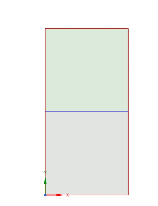
The geometry modelling of the problem is done in the space-claim pre-processor in which two surface with unit thickness of 20mm x 20mm are constructed. The water surface is made at top of the air surface. As the simulation is 2D and geometry is very simple we can adapt the conformal mesh with hexahedral element type. To make sure conformal mesh present for simulation it is important to have geometry topology as shared. In which the common edge between two surface are shared with each other. This can be done by using share topology option in space-claim which will create a common interface between the two geometry.

• Meshing

After completing the geometry for simulation, the discretization of geometry is required to calculate the governing equation on the discretize volumetric domains. As the geometry is way more simple there is no need to apply any local control for the meshing. If user want he can use face meshing local option to just refine the lines of mesh. For each case the mesh size is lowered to capture better mixing of fluid caused due to instability of interface. For the baseline simulation which is case 1, mesh size used is 0.5mm. The mesh will look like:

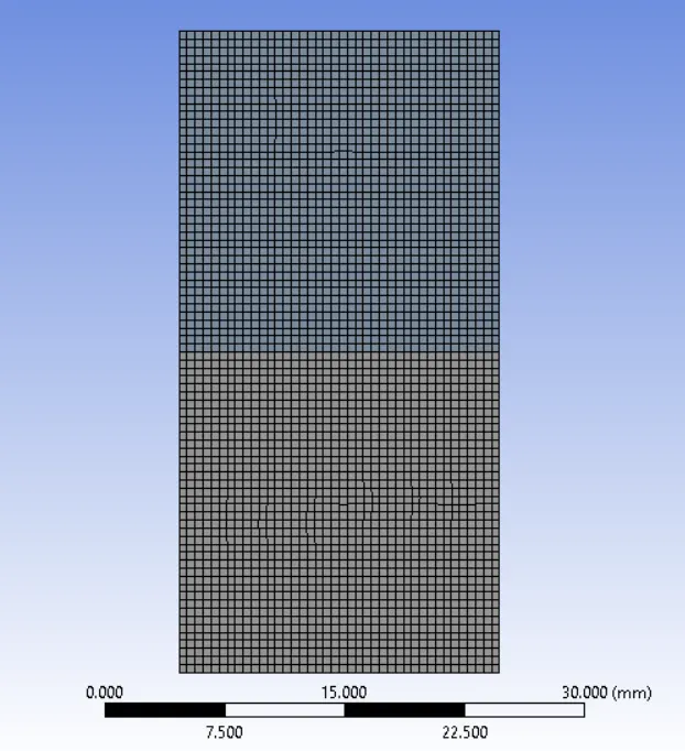
For this case of simulation there is no need of creating any boundary condition as we are trying to simulate liquid under the gravitation effects. As there is interface is already created between two different fluids there no requirement of creating any Mesh interface or Markers for simulations.

• FLUENT Setup

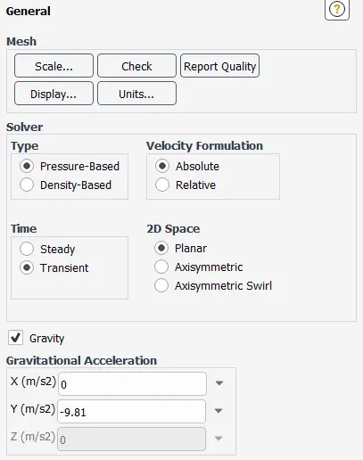
The FLUENT setup is very simple without consideration of any boundary conditions. The important things which need to be consider while making the setup are application of gravity for simulation, defining fluid property of water, creation of multiphase model using volume of fluid method and patching the phase with respect to volume fraction. The defining of gravity can be done from general setup FLUENT in which gravity will be applicable in negative Y direction with amount of 9.81m/s. The simulation will be transient in nature and pressure based solver is used because of instability is mainly created due to pressure disturbance. The image of general setup is shown below:

Before setting up the multiphase model it is important to provide secondary fluid property in the FLUENT. Setting up multiphase model can be done before providing the fluid property but it is better practice to go with standard model. The water as secondary fluid can be setup by using material section in ANSYS FLUENT in which both solid and fluid material are defined in database. From the database we can select the water as fluid and provide it to simulation. The Water and Air as fluid and their property are given below:

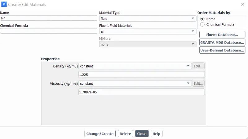
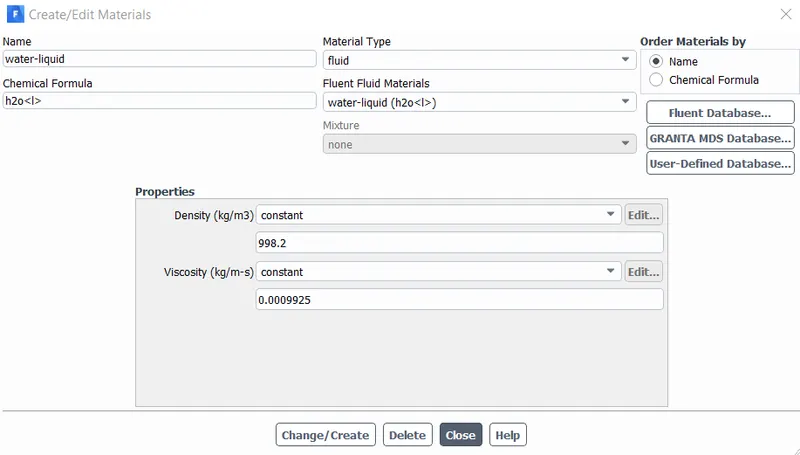
for the baseline mesh and for other three cases we are going to use default fluid property and for last case we will use the user defined material. After completing the material definition, the multiphase property has to be provided for simulation. This can be done in setup model where we can choose turbulence model. There we can see the multiphase option in which further we need to select VOF method. This is shown in below image

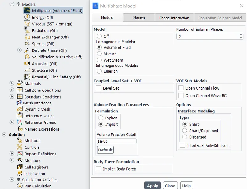
The formulation which can be choose for VOF model are explicit and implicit. For this simulation we are going with implicit approach as explicit approach is mostly use with interface where surface tension and compressibility is dominant, also implicit formulation is used for most of cases where gravity effects are dominant and it solves phase continuity equation iteratively with momentum and pressure. After defining the method for multiphase model further it is necessary to select the phase involve in simulation which can be done in another tab for multiphase model. As we have selected the number of Eulerian phase as two, we need to have two different fluids. The primary phase is selected as Air and secondary phase is selected as Water which are shown below:

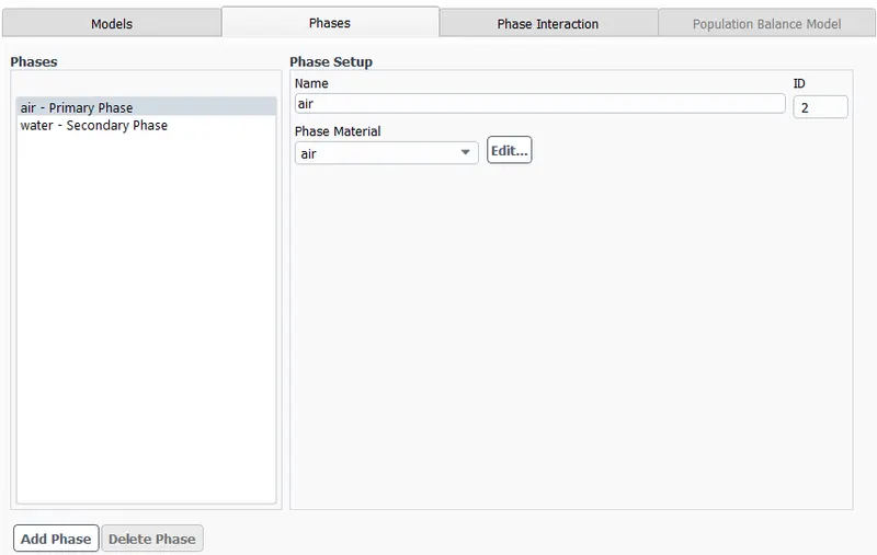
There is no requirement of defining phase interaction between fluid because we are not considering any surface tension variable or heat and mass transfer between the fluids. The interface modelling is also considered as sharp because we have distinct interface between the fluid. The dispersed interface modelling is used when the phases are completely mixed. After making sure that phases are defined properly there is no need to make changes in solution method as when selecting VOF method FLUENT automatically enable PRESTO as pressure-velocity coupling scheme for problem. As PRESTO is mostly selected for pressure-based solver where gravity and pressure are dominant variables.

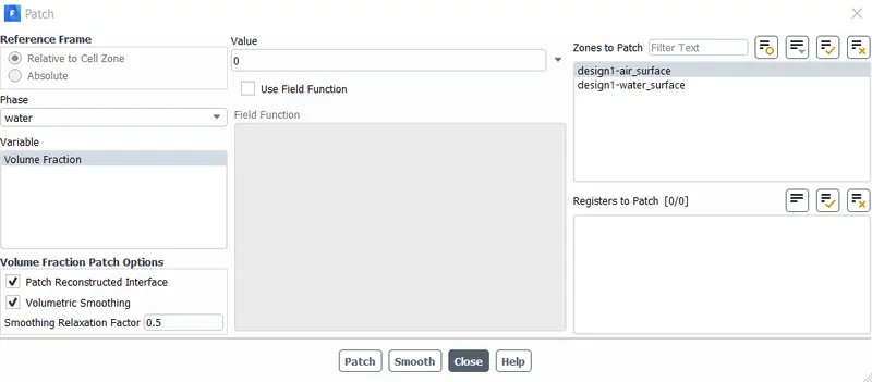
Patching in the FLUENT can be considered as initial conditions for VOF method, where user define the amount volume present in the domain. In general cases primary and secondary phases can be defined arbitrarily, for most of cases it is common practice to provide dispersed phase as secondary phase and primary phase as compressible ideal gas. Patching can be only done after the solution initialization, if user make initialization after solution completion for another case it is important to patch domain again as data get erased after each initialization process. The patching for water and air as domain is shown as:

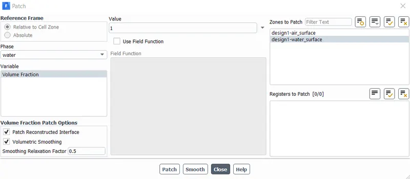
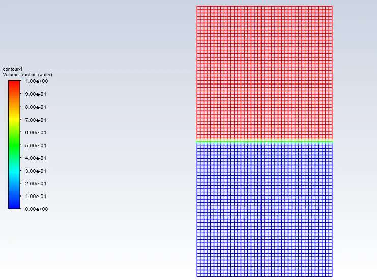
After applying the patch to the domain it is necessary to see whether it is clearly patch the domain or not. This can be done be creating contour of volume fraction of water in post-processor. In which volume fraction as 1 to 0.5 is representing water and 0.5 to 0 representing the air as domain fluid. This is shown below:

After applying the patch there is only need to do the calculation for simulation with suitable time step and number of iteration required. It is better practice to see the simulation when it is performing the calculation this can be done by the simulation animation of the volume fraction contour. The time step size for the simulation is 0.005 and the number iteration will be changing as per the mesh size. For the baseline mesh setup, the number of iteration required are about 650. For post-processing the result and see the clear animation it is important to create the data files of result which can be further access in result of ANSYS FLUENT.

CASE 1: - 0.5MM MESH SIZE

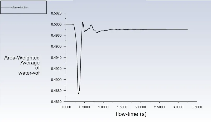
For this case we are going to use the mesh size as 0.5mm which will create total number elements which are 3200. The results for the simulation are given below:

1) Volume fraction of Water

2) Animation link for Volume fraction

https://drive.google.com/file/d/1Rq7hRwI7KQwL5p2MNQQUn_dcaw6Fm3d_/view?usp=sharing

3) Volume Fraction of Water Youtube link

CASE 2: - 0.25MM MESH SIZE

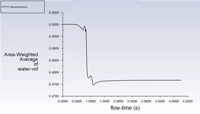
In second case we reduce the mesh size by half and perform the same process of setup for each case. The number of elements created in this case are 12800.

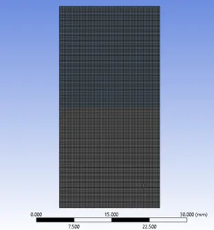
This case setup has been run for similar time step with 850 iterations. It was observed in previous simulation that 650 iterations are not enough to capture whole mixing of liquids. The results are shown below:

1) Graph of Volume Fraction of Water

2) Animation of Volume Fraction Drive Link

https://drive.google.com/file/d/16fpQPzJ0U7eIPZ90XbIEJO-mlBO6dIq6/view?usp=sharing

3) Animation of Volume Fraction Youtube

CASE 3: - 0.1MM MESH SIZE

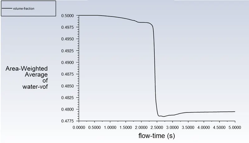
For the third case we will reduce the mesh size to 0.1mm and see the effects of mixing during instability. For this case the number element was created are 80000. The result is shown below:

1) Graph of Volume fraction of water

2) Animation of Volume Fraction of water Drive link

https://drive.google.com/file/d/12nN1hN607tZE2aGheodpfNWRCpsQo5sU/view?usp=sharing

3) Animation of Volume Fraction of water Youtube Link

CASE 4: - 0.1MM MESH SIZE WITH USER DEFINED MATERIALS

For this case we are going to use the same mesh size but will use the user defined material and water as default material. The property of UDM is shown below:

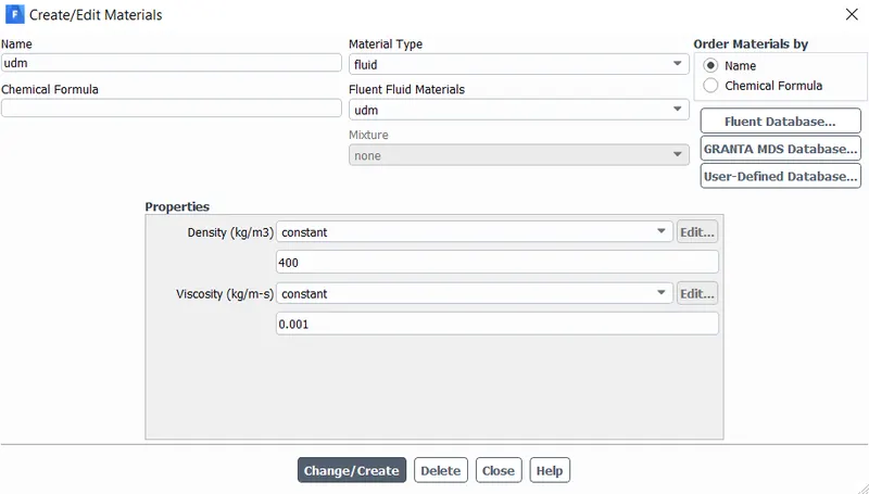
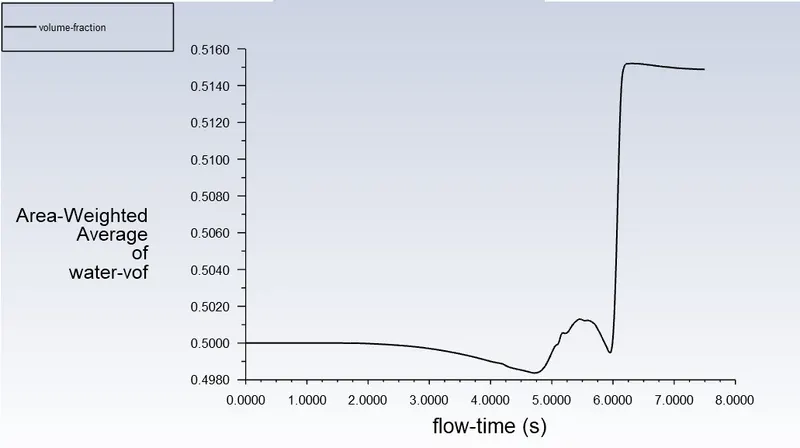
The simulation is run for almost 1500 iteration and the result were shown below:

1) Graph of Volume fraction of water

2) Animation of Volume fraction Drive link

https://drive.google.com/file/d/1hb6LlnQ3wtyvKBrL4P_sHKFUaDSWFjTW/view?usp=sharing

3) Animation of Volume Fraction Youtube link

Please have some patience while watching video as it was made for 0.1mm mesh size.

Atwood Number: -

Atwood number is the non-dimensional number which is used for the study of hydrodynamic instabilities in density stratification flows. The Atwood number is given as:

`A=(ρ1-ρ2)/(ρ1+ρ2)`

Where,

ρ1 is the density of heavier fluid and

ρ2 is the density of lighter fluid.

Atwood number for Case No. 1, 2 and 3

Density of Heavier fluid (water) = 998.2 kg/m³

Density of Lighter fluid (Air) = 1.225 kg/m³

^{`A=(998.2-1.225)/(998.2+1.225)=0.9975`}

Atwood number for Case No. 4

Density of Heavier fluid (water) = 998.2 kg/m³

Density of Lighter fluid (Air) = 400 kg/m³

^{`A=(998.2-400)/(998.2-400)=0.427`}

Conclusion: -

• Why not steady state solver:

The VOF model are generally used to solve the time dependent problem but we can also solve the steady state simulation. A steady state simulation of VOF model is only sensible when our solution is independent of the initial conditions and there are particular inflow and outflow boundary conditions are presents for individual phases. Steady state solver is only used when the results are required at the end of time step and no requirement of intermediate phase results. In case of instability it is important to make sure volume fraction as the function of time as it will change with respect to time.

• Effect of Mesh on Results

From the result of volume fraction graph with respect to time we can see the drop of area weighted average of volume fraction for water is earlier in baseline mesh setup and as the mesh size is decreasing the drop get moving forward in time, this shows that as the number of element are increased we are getting better capture of flow phenomenon. Hence we can say that mesh size effects the convergence of hydrodynamic instability. Also it was noticed that as the mesh size is lowered the number of iteration to perform the simulation has been increased by factor of 2.5 – 3.

• Comparison of Atwood number

For case 1, 2 and 3 we are seeing Atwood number closer to 1 and for the case of user defined material it is almost reduced to half. When Atwood number is close to 1 we can see the stratification effect at more level which means mixing is symmetric in nature. For case of user defined material as we have increased the density of material the mixing effects are lowered and only small plateau can be seen from simulation.

• Comparison of Animation

For case 1 it was very evident that lack of mesh elements results in very fast mixing and quick gaining of equilibrium position by both of the liquids. In second case we can see that the mixing is slowed down and number of iteration to complete the simulation has been increased as well. In third case the mixing is very slow and we can see better resolution of how water is making it way downward due to gravity. In fourth case, the user defined material has been introduced. In this case we can see the formation of mushroom shape when water is stared interacted with user defined material.