Week 3: Flow over a backward facing step
Challenge 2 – Backward Facing Step Simulation
Aim: - Simulation of Backward facing step flow in converge software with different mesh grid values.
Objective: -
- To study the importance of simulation for backward flow step in turbulence modelling.
- To case setup the backward flow step with creating the geometry in Converge Studio software.
- To run the simulation for three different mesh size i.e. 2mm, 1.5mm and 1mm.
- To post process the result in the paraview and showcase pressure and velocity contour for three mesh size.
- To get the plot of velocity, pressure, mass flow rate and cell counts from the Converge Studio for 3 different mesh size.
- To explain the result and reason behind flow separation in the flow filed.
Introduction: -
Backward flow step problem is mostly used in evaluation of different turbulence model. Turbulence models are developed to capture the exact nature of flow when Reynolds number are more than limit for internal flow. In the backward flow setup, the flow gets detached from the flow domain and cause increase in negative pressure which further results in recirculation domain neat the step.
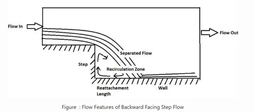
From the above figure, it can be see that the recirculation zone is created after the flow past step. The amount of negative pressure develop in that recirculation region is depend upon the velocity and flow and height of step. It is important to study the recirculation zone in such cases as the effect of cavitation is increased which further lower the life of metal when come in contact with such phenomenon. The fully developed flow entering domain from the left hand side. After the step there is sudden expansion which cause the pressure gradient to emerge which detaches the and recirculation zone get formed.
The separation and reattachment of the turbulent flow are occurring in many practical applications. It is seen in many diffusers, combustors and channel with sudden expansion and in external flow like flow around the airfoil of planes. In such situation, the flow experience an adverse pressure gradient, which cause the separation of boundary layer from solid surface. The flow will get reattach downstream of domain forming a recirculation bubble. The presence of separated flow and together with reattaching flow gives rise to increased unsteadiness and pressure fluctuation which cause vibration and noise generation.
To know whether the flow is turbulent or not, it is important to calculate the Reynold’s number which is given as:
`Re=(ρ ×V ×D)/μ`
Where,
ρ is the density of fluid in kg/m3
V is velocity of fluid in m/s
D is the hydraulic diameter as flow is flowing through rectangular shape in meters
µ is the dynamic viscosity in kg/m-s
For the simulation, the flow is governed by pressure difference hence it is necessary to calculate the velocity with which fluid is entering into domain. This can be calculated using the relation between the static pressure and the dynamic pressure which is given by:
`P_(static)=P_(Total) {1+ (γ-1)/2 ×M^2 }^(-((γ-1)/γ) )`
where M is the Mach number which is further given by:
`M=v/a`
`a= √γRT`
Rewriting equation
`P_(static)=P_(Total) {1+ (γ-1)/2 ×v^2/γRT}^(-((γ-1)/γ) )`
The total pressure at the inlet boundary is 110325 Pascal’s. For the initial pressure it can be treated as 101325 Pascal’s.
`(101325/110325)^((-1)/3.5 )= {1+(1.4-1)/2 ×((V^2 ))/(1.4*287.05*300) }`
`V=109.80 m/s`
The calculation of hydraulic diameter is given by following equation:
`D=(2BC)/(B+C)`
Where,
B is the width of inlet which is 0.025m
C is the height of inlet which is 0.00854m
Therefore, the hydraulic diameter is calculated as:
`D=(2*0.025*0.00854)/(0.025+0.00854)=0.01273 m`
The Reynolds number is calculated as:
`Re=(1.177*109.80*0.01273)/(〖1.84e〗^(-5)) =89410.677`
From the equation it is seen that the Reynolds number for flow is greater than 4000 for internal flow, hence the flow is turbulent in nature.
Case Setup: -
The backward flow step simulation is turbulent flow simulation because of high Reynold’s number. In some cases, this kind of simulation are much time consuming and retrieving the exact flow characteristics are difficult. Hence, sometimes this simulation can be treated as pseudo-transient in which steady state simulation is carried out with higher time duration to reach the steady state of flow. In the case setup the simulation is address as transient in nature. The geometry is provided but it was built in the converge studio. The dimension of the geometry is given below:
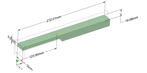
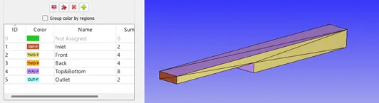
After creating the geometry, it is necessary to create the boundary for each of the surface in the geometry. The boundary which are used in the simulation are inlet, outlet, 2D wall and top & bottom walls. The geometry is representing as 2D in nature as front and back face are treated as infinite in length. The boundary with different color is shown in figure:
The material for the simulation is selected as ‘Air’ with the species O2 and N2 in species settings. The global transport properties are kept same as default and rest of the things were treated as constant. After setting up the material selection, simulation parameters were selected in which solver is treated as steady state with full hydrodynamic mode as gas flow solver is consider as compressible in nature.
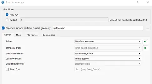
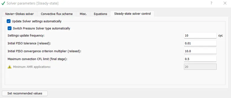
After selecting steady state simulation, it is necessary to create the steady state monitor to actually treat the simulation as steady state in nature or else solver will see it as transient in nature. For steady state monitor Average Velocity and Total Pressure are selected as monitor parameter at the outlet of geometry. The solution has been set up for 15000 cycles with 2 seconds as maximum time step. The care should be taken at the setting up the value of Maximum convection CFL limit for the simulation which should be in between 0.1 to 2. This setting is make the simulation over-relaxed or under-relaxed depend upon the number entered by user. By default, for version 3.0 this number raise to 10 which by default over-relaxed in nature and user will never get the true results. Similar to time setting it is necessary to select the pressure velocity coupling scheme for the simulation which is PISO and the pressure based solver is used for problem. Another thing which is need to be considered in simulation is setting of steady state solver control in which again Maximum Convection CFL limit has to be equal which has been set previously in Simulation time parameters setting or lower than it. For this problem the limit is set as 0.5.
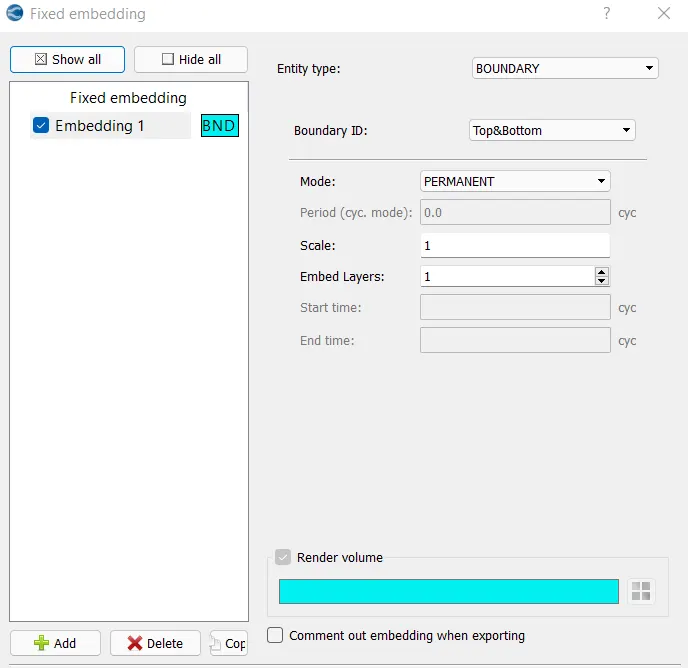
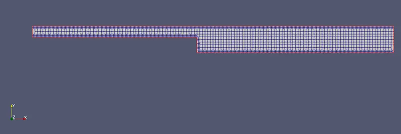
Sometimes it’s better to create regions for the simulation before setting up the boundary conditions. As eventually user need to come back in the boundary condition to set up the region selection for particular boundary condition. In region and Initialization user need to add the new Region which can be renamed. The region should have initial pressure and temperature entered with species mass fraction values. After completing the creation of region, the boundary conditions are need to be set. For the inlet ‘INFLOW’ boundary condition is selected with total pressure of 110325 Pascal’s with the air as working fluid. The front and back boundary are treated as 2D stated earlier. The Top & Bottom boundary is selected as WALL with no-slip wall treatment. The outlet of geometry is considering as ‘OUTFLOW’ and the total pressure is equal to initial pressure i.e. 101325 Pascal’s. For the turbulent boundary layer separation phenomenon, the RNG K-epsilon model is used with standard parameter. For such simulation most probably K-omega SST 1 equation model with omega in integral term are selected for capturing the Brownian motion of particles. The main aspect of the simulation is to run for three different grid conditions which is 2mm, 1.5mm and 1mm mesh size. It is important to capture the motion near the boundary of top and bottom, for which inflation layer need to be provided. In case of Converge Studio this can be done by using Fixed Embedding in which the boundary is selected as Top & Bottom and permanent embed layer of 1 is selected. Depend upon the user computational strength this can be varied accordingly.
After completing the grid setup, the remaining of case setup is to select the post variables which are most probably for steady state simulations are density, pressure, temperature and velocity with number of cell counts. In the post variable selection, the user should not forget about setting up the mass fraction in the species tab where O2 and N2 species has to be enter. In output files the result files iteration for 3D output can be selected which is set to be 100 and restart files is set as 1000 cycles.
Results: -
Case 1 - Mesh Size = 2e-3 Meters
1) Mesh
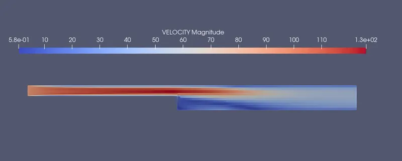
2) Velocity Contour
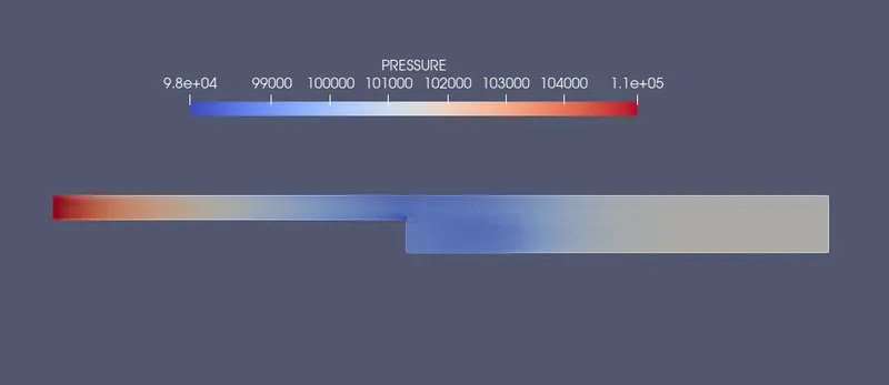
3) Pressure Contour
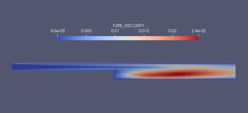
4) Turbulent Viscosity
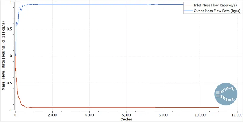
5) Mass Flow Rate Plot
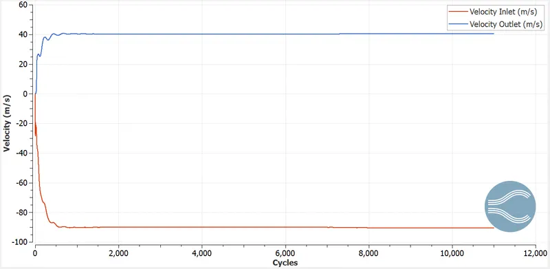
6) Average Velocity Plot
7) Pressure Plot
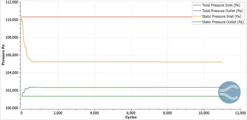
8) Total Cells plot
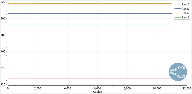
9) Animation Link for Velocity Contour
10) Animation Link for Pressure Contour
Case 2 - Mesh Size = 1.5e-3 Meters
1) Mesh
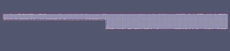
2) Velocity Contour
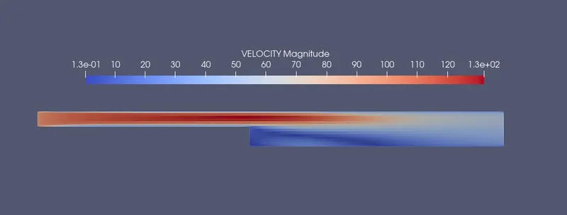
3) Pressure Contour
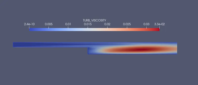
4) Turbulent Viscosity
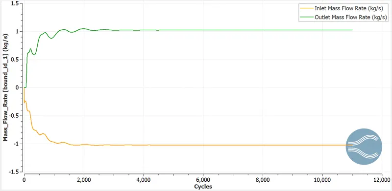
5) Mass Flow Rate Plot
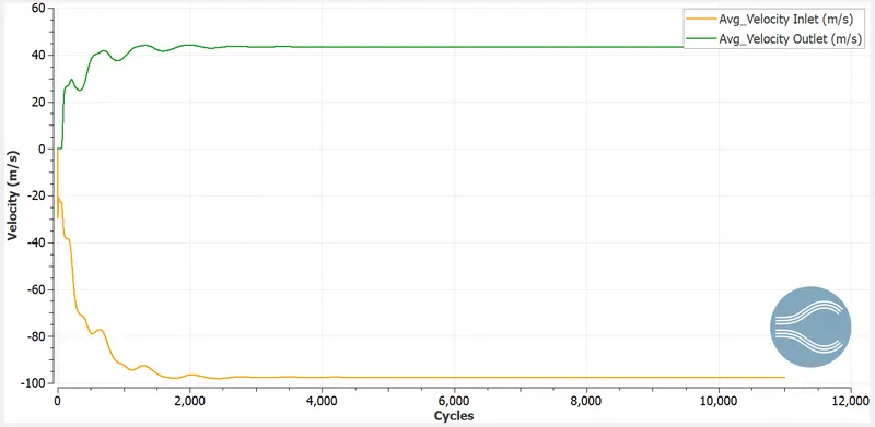
6) Average Velocity Plot
7) Pressure Plot
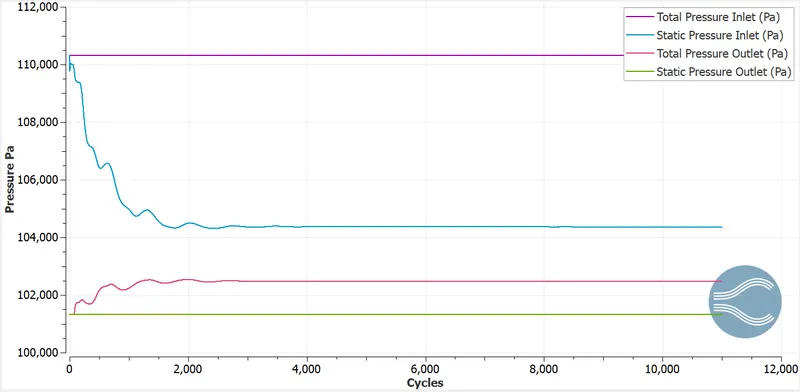
8) Total Cell Plot
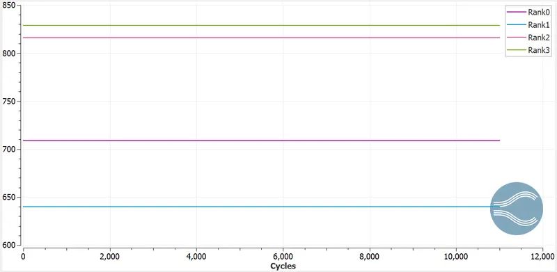
9) Animation Link of Velocity Contour
10) Animation Link of Pressure Contour
11) Animation Link of Turbulent Viscosity
Case 3 - Mesh Size = 1e-3 Meters
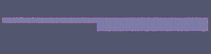
1) Mesh
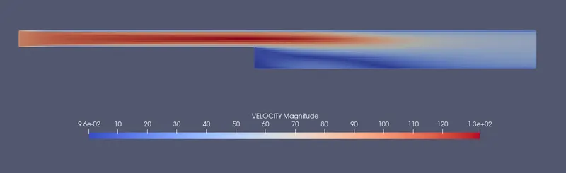
2) Velocity Contour
3) Pressure Contour
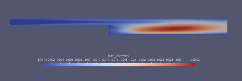
4) Turbulent Viscosity Contour
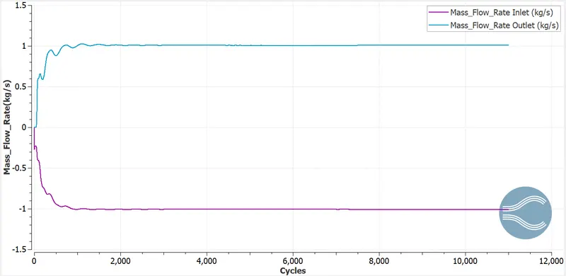
5) Mass Flow Rate Plot
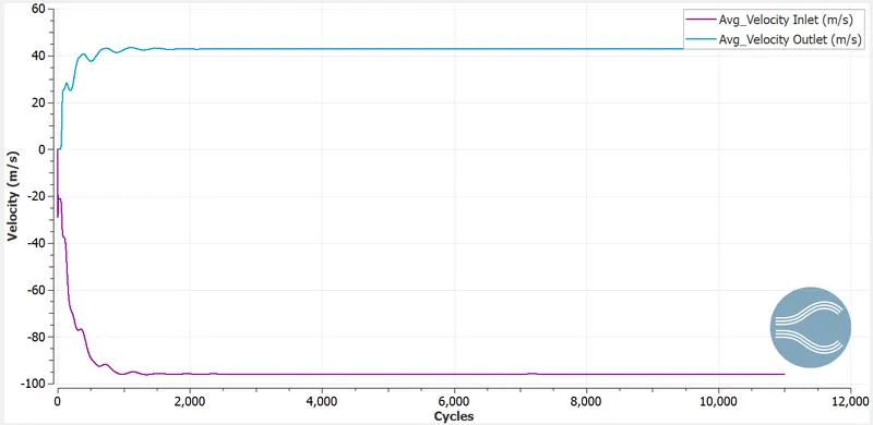
6) Average Velocity Plot
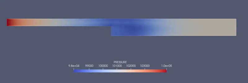
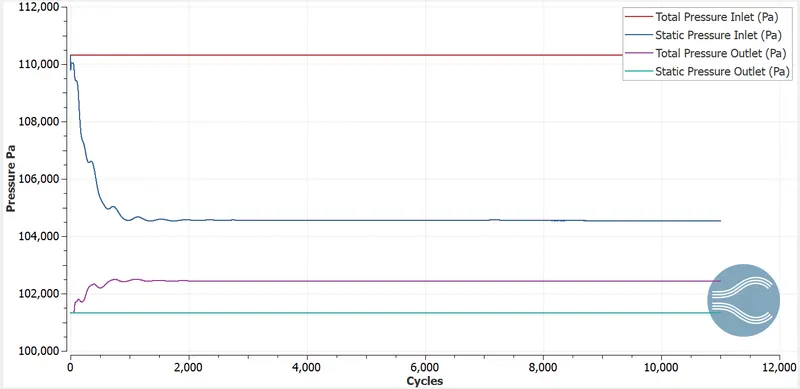
7) Pressure Plot
8) Total Cell Count
9) Animation Link of Velocity Contour
10) Animation Link of Pressure Contour
11) Animation Link of Turbulent Viscosity
Observation: -
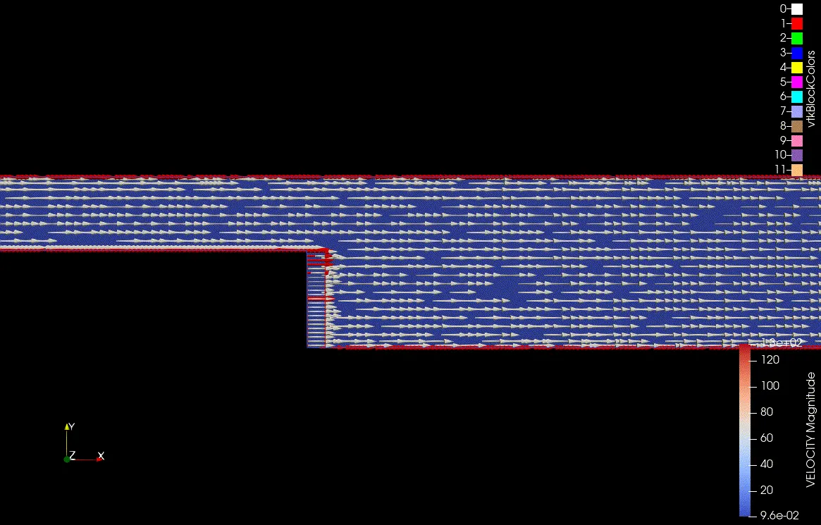
1) From the results it can be seen that flow detach after the sudden expansion of domain due to step. This causes the flow to separate from main flow and then reattach further in domain.
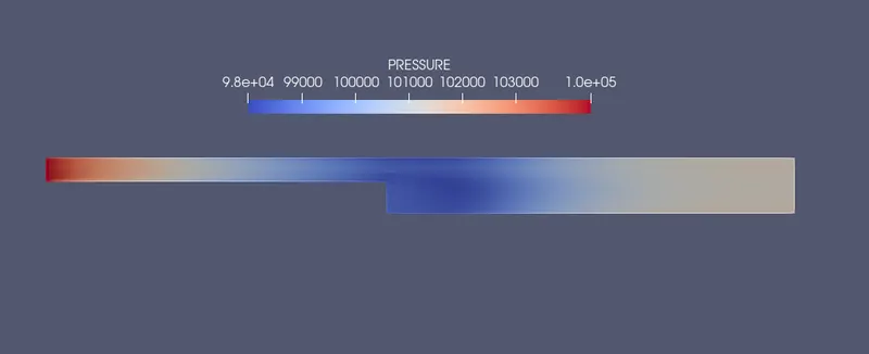
2) Because of Separation in the vicinity of step velocity get lowered which result in creation of vortices in the zone. From the pressure contour it can be seen that, the pressure has drop significantly which result in pressure drop of around almost 1700 Pascal's.
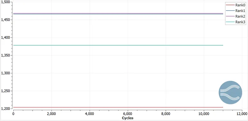
3) From all plots it can be seen that flow has stabilize after 2000 iterations. Increase in number of mesh size provide better contours also the result near the wall has been enhanced.
4) In the velocity contour the inlet velocity ranges from 107 to 109 m/s which is similar to which has been calculated from analytical solution.
Project Link : - https://skill-lync.com/student-projects/backward-flow-step-simulation-in-converge-studio-3-0