Week 10 - Simulating Combustion of Natural Gas.
Combustion Simulation of Natural gas inside a Burner using ANSYS FLUENT.
Content
AIM
Objective
1.0 Introduction
1.1 Opening Remark
1.2 Solution Approach & Methodology
2.0 Pre-Processing
2.1 Geometry clean-up
2.3 Meshing & Named Selection
3.0 FLUENT Setup
3.1 Viscous Model Setup
3.2 Species Model Setup
3.3 Specification of Boundary conditions
3.4 Solution Methods
4.0 Simulation Results
4.1 Baseline Mesh setup results
4.2 Case 1 – Oxygen 5%
4.3 Case 2 – Oxygen 10%
4.4 Case 3 – Oxygen 20%
4.5 Case 4 – Oxygen 30%
5.0 Inference
5.1 Result table
5.2 Conclusion
5.3 References
AIM: -
Combustion Simulation of Natural gas inside a Burner using ANSYS FLUENT.
Objective: -
- To study the combustion Phenomenology for the whole problem.
- To study the eddy dissipation model.
- To study the NOx and soot formation inside the burner.
- To pre-process the geometry for the simulation.
- To select correct element size and type for the simulation.
- To setup the combustion simulation using eddy dissipation model.
- To setup NOx and soot formation model in simulation.
- To plot the mass fraction of CO2, H2O, CH4, N2, O2, NOx and soot formation.
- To perform the simulation by adding water with fuel in range of 5% to 30% to lower the NOx and soot formation in combustion.
1.0 Introduction
1.1 Opening Remark
A combustion is the Exothermic chemical reaction of a fuel with an oxidant to form the product. Basically there are two type combustion one is flame mode in which the thin zone of intense chemical reaction called ‘flame’ exist and another one is Non-flame mode in which volumetric combustion process is exited. The combustion simulation is performed to get the predictions of:
- flow fields and mixing characteristics
- Temperature fields
- Species Concentrations
- Particulates and pollutants.
The application of combustion modelling is applying for various kind of reacting flows such as furnaces, boilers, Process heaters, Gas turbines, automobiles and Rocket engines.
Modelling of combustion reaction in a software is difficult and need to take care for species which are taking part in reaction and its products. The combustion CFD model comprises of chemical kinetics and similarly achieving reacting flow mixture environment. Considering chemical kinetics, it is also important to have properly defined physical model with simulation to get the maximum out of process. Computational fluid dynamics of combustion model should be capable of enough to provide information related to species concentration, their volumetric generation or diffusion rate and changes in the system parameters like enthalpy, temperature and mixture density. The similar model should be good enough to solve the general transport equations for fluid flows and heat transfer as well as additional equations of combustion chemistry and chemical kinetics incorporated as per simulation environment details.
Chemical kinetics is part of combustion phenomenon, which is the study of entire reaction mechanism subject to different operating conditions. The whole reaction mechanism is the overall reaction of fuel and air with the elementary reaction. The elementary reaction is consisting of intermediate reaction cause generation of intermediate species, and the species react with fuel and air will cause the elementary reaction. This intermediate reaction caused due to breakup of chain reaction of fuel and air. The chemical kinetics is important as it provide when combustion process is going to start i.e. time period of ignition delay, rate of work done and used to determine emission from the chemical reactions. The elementary reactions in the case any combustion phenomena are mostly of three types which are bimolecular reactions, unimolecular reactions and thermolecular reactions. In bimolecular reaction the reactants produce the product and same product can be undergoing to produce the reactant. This reaction is most common in combustion. In unimolecular reaction there are two types one is isomerization in which transformation of composition is occurred and another case is decomposition in which breakdown of composition is occurred.
1.2 Solution Approach & Methodology
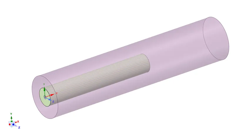
The geometry which is provided for the problem is 3D in shape. The simulation approach which used for the problem is 2D Axi-symmetry steady state turbulent model with species transport equation. The use of 2D Axi-symmetric model reduce the work load on the computational source and will reduce the time required for simulation. The burner geometry in 3D shape is shown below:
|
Figure 1- 3D View of Burner |
|
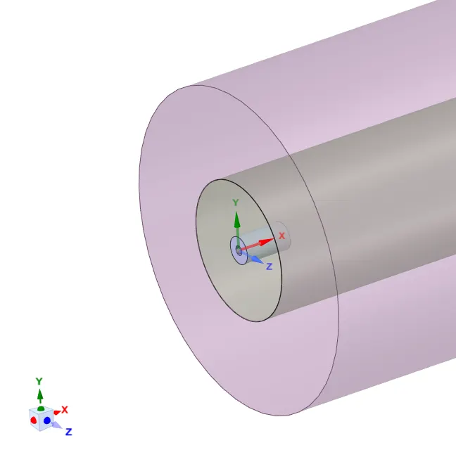
Figure 2- 3D Expanded view of Burner Fuel Opening |
From above two geometries we can see the three different solid inside of each other. As the solution point of view the fuel is entering from the opening diameter of 3.3mm and rest is the air entering in chamber. Whole geometric pre-processing will be discussed in later section. The flow air and fuel is considered as turbulent in nature. The species model which is used for simulation is species transport and reaction time is volumetric. The mixture material used for the whole simulation is methane-air-2step in which basic species with water has been seen as the reactants. The mixture material carries some information with them which is stored in FLUENT, that information’s are:
- list of constituent species, referred to as ‘fluid’ materials
- it contains list of mixing laws which provide how mixture properties to be derived from the properties of individual species.
- diffusion coefficient for individual species
- material properties like absorption and scattering coefficient which are not associated with individual species.
In combustion process most of the fuel are fast burning and the overall rate of reaction is controlled by mixing caused due to turbulence. In non-premixed flames, turbulent cause the fuel and oxidizer to mix and convert them into reaction zones where it burns as quickly as possible. Similarly, turbulence also mixes the cold reactants and hot products into the reaction zones, where reaction happen rapidly. Hence for pre-mixed combustion eddy dissipation model can be used to create the reaction into chamber. This model is only applicable for turbulent flows only. It assumes the reaction is fast relative to the transport processes in the flow. The reaction rate is proportional to turbulent mixing time defined by kinetic energy (k) and it dissipation rate epsilon (ɛ).
The formation of NOx and soot are due the incomplete combustion or due to excess amount of fuel inside the chamber. The formation of soot is also depending on the temperature of reaction. If the temperature of reaction is not high enough to produce the product of reaction, then formation of soot is occurred. The NOx emission can be formed through series of mechanism during both the premixed and diffusion burning. As in methane-air-2step mixture for the baseline setup the fuel present in higher quantity which rises to creation of NOx and soot in the chamber. To capture the effect of NOx and soot in the burner the FLUENT have NOx and Soot model which incorporate with eddy dissipation model of species transport. For determining the NOx FLUENT has different pathways in which NOx formation is occur during the combustion process. The pathways are Thermal NOx, Prompt NOx, Fuel NOx and NO2 intermediate. In case of Thermal NOx is depend upon highly temperature dependent chemical reactions. The Prompt NOx formation is proportional to number of carbon atoms present per unit volume and independent of parent hydrocarbon identity. The creation of Prompt NOx is most prevalent in rich kind of flames reactions. The main source of Prompt NOx is from the fuel fragmentation in hydrocarbon flames and the major contribution is CH and CH2. Hence it is important to check the Prompt NOx pathways to determine the generation of NOx in combustion reaction. Beside of Thermal NOx and Prompt NOx the fuel NOx also contribute in creation of major NOx. The nitrogen-containing organic compounds present in the liquid or solid fossil fuel which contribute for the formation of NOx during combustion process. Similar to NOx the soot formation is also incorporated in the simulation by one-step method.
All above methods are used to make the combustion simulation for the given burner problem. The boundary conditions are discussed in further section. The solution methodology is divided into five case. In which the baseline mesh setup is used to determine the creation of NOx and soot inside the burner. As the NOx and soot are not favorable for the outside environment it is better to lower to such extent which are defined by the environmental norms by government. To lower the NOx and soot formation the water is added with fuel in 5% to 30% amount. According to it rest of the 4 cases are defined. The overall cases are given below, all the fuel and water are defined in mass fraction.
Case 1 – Baseline Mesh setup.
Case 2 – Combustion simulation with Fuel = 0.95 and Water = 0.05 (5%)
Case 3 – Combustion simulation with Fuel = 0.9 and Water = 0.1 (10%)
Case 4 – Combustion simulation with Fuel = 0.8 and Water = 0.2 (20%)
Case 5 – Combustion simulation with Fuel = 0.7 and Water = 0.3 (30%)
Using this case setup, the formation of NOx and soot is compared with percentage of water provided in the burner with fuel. The results will be plotted for mass fraction of different species in the burner at different locations.
2.0 Pre-processing
The pre-processing of the whole setup is done space-claim geometry modeler and workbench of ANSYS software. The pre-processing includes geometry clean-up for meshing and further simulations. As discussed earlier in solution approach the model will treat as 2D Axi-symmetric model, henceforth the 3D geometry has to be change.
2.1 Geometry Clean-up
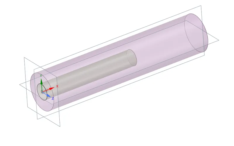
The geometry clean-up is done for the burner 3D model. As it required to create 2D model from provided geometry of burner. The model will directly open in space-claim design modeler and planes are created at the center point of geometry which is shown in below:
|
Figure 3- Creation of Plane at Centroid of Geometry |
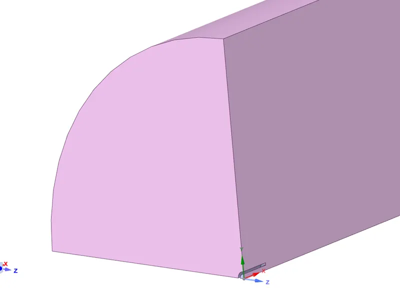
Creation of plane allows to split the body in half or in quarter portion. As for 2D Axisymmetric model it required to cut in quarter model and then the face of that quarter section is copied and pasted in new design. Before copying the face of quarter section, it is required to combine the two section of geometry which are present in whole assembly. Both the geometry instead of fuel opening area can be treated as one body. After creation plane the split body option from space-claim design tab is used to cut the body in half first parallel to XY plane and then it need to be cut parallel to ZX plane. After completion of both splitting only quarter part is required rest of part need to be deleted. The quarter section of geometry is shown in figure 4:
|
Figure 4- Quarter Section after body split command |
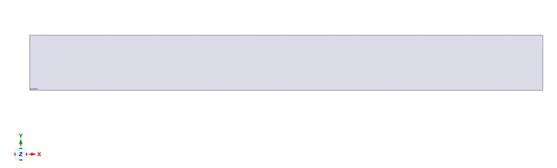
From the quarter section shown in figure 4, the front face of geometry can be used for simulation. To have the face for simulation it is necessary to select the face and copy it. After copying the face from geometry, it has to be pasted in new design which can be made from File>New>Design option. The geometry must be pasted only in XY plane for the sake of Axi-symmetric approach. Figure 5 shows the final geometry for simulation.
|
Figure 5- Final 2D section Front View |
2.2 Meshing & Named Selection
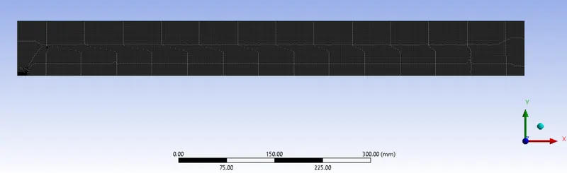
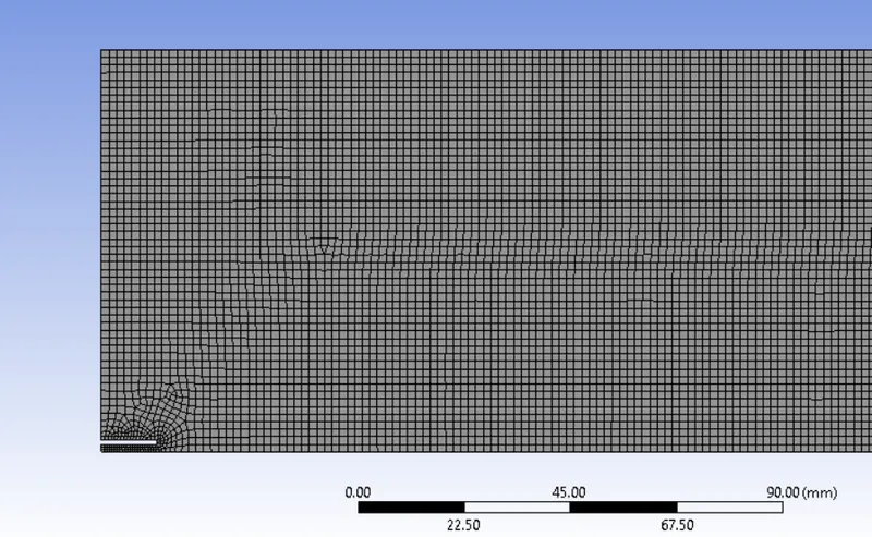
As the geometry is 2D in nature, the number of element required as compared to 3D model will be less. The mesh should be fine enough to caught every details of species and their reaction inside the chamber. The type of element which is used for meshing is Quad 4. Because of simplicity of geometry and accuracy of solution required, it is best practice to go with quadrilateral elements. The method used for the meshing is Automatic method in which Quadrilateral dominant method has been used. In the geometry there are some irregularity which cause element to reshape in zone of vicinity. The proximity size function is used for providing element in the smaller zones of geometry. The proximity size function requires number cell across the gap in geometry. As there is only one possible gap in geometry near the left hand bottom side and it is necessary to create more number of element near the fuel inlet. The number of cell in the gap is provided as 3 and the element size of 1.6mm is used for whole geometry.
|
Figure 6- Mesh for Simulation |
|
Figure 7- Expanded View of Mesh |
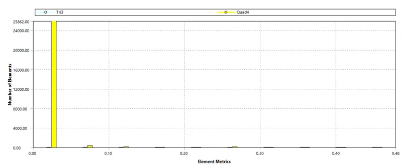
The element quality for overall mesh setup is in best condition. The maximum skewness for the mesh is 0.48 and the maximum aspect ratio 1.62. The orthogonal quality of mesh is just opposite to skewness.
|
Figure 8- Skewness Mesh Quality |
From figure 8 it is seen that two element types are used for mesh which are triangle 3 node and quadrilateral 4 nodes. The Quadrilateral dominant mesh type create quadrilateral element in most of the part of geometry where it could not make quad 4 elements it will try to create triangular element. For boundary condition in FLUENT it is necessary to create name selection in workbench. As the combustion process require both air and fuel for chemical reaction. There are two inlets and one outlet. The inlets are treated as velocity-inlet and outlet as pressure outlet. The small edge at left hand bottom corner of geometry is considering as fuel inlet and rest of the edge after gap is consider as air inlet. The right hand side extreme vertical edge is considering as outlet and bottom edge is considering as axis for simulation, rest of the edges are considering as wall. The following figures are showing named selection for whole simulations.
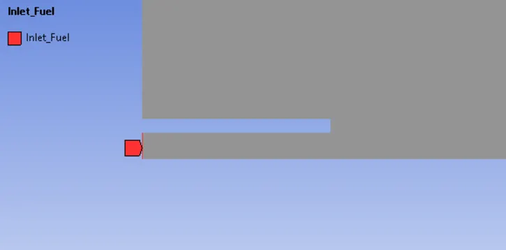
|
Figure 9- Fuel Inlet Named Selection |
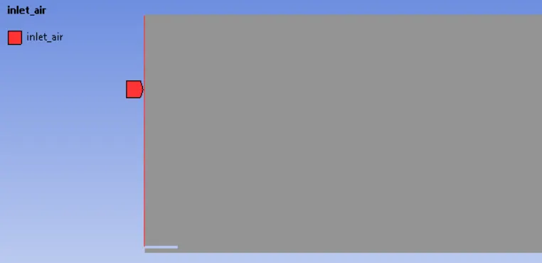
|
Figure 10- Air Inlet Named Selection |
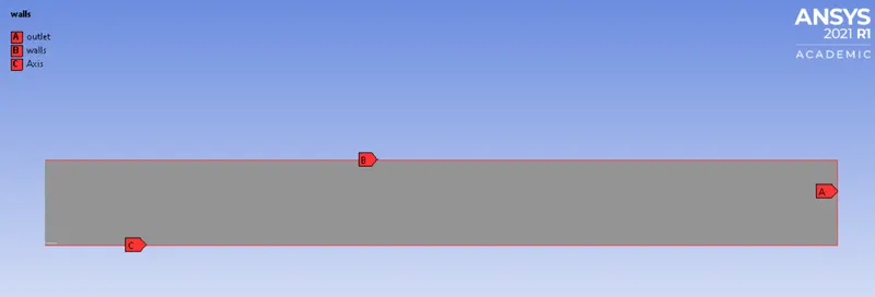
|
Figure 11- Other Named Selection |
3.0 FLUENT SETUP
FLUENT setup and solving the required problem is the part of pre-processing. In this section the different part of setup is discussed in which viscous model setup, boundary conditions and solution method setup are involved. The general setup required for simulation is pressure based steady state approach for problem. The gravity is not enabled for the simulation. Figure 12 shows the general setup of FLUENT.
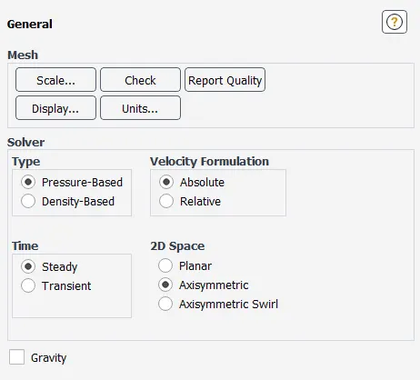
|
Figure 12- General Setup for FLUENT setup |
3.1 Viscous Model Setup
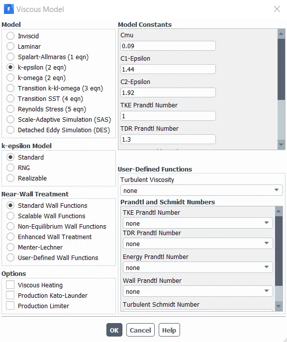
The viscous model setup comprises of information about setting up required flow characteristics for the problem. As state earlier in solution approach of the problem that, flow will be turbulent in nature and species transport equation is need to be solved using eddy dissipation method. In the same context k-epsilon turbulent model with standard wall function are used as input for the flow phenomenon. As per the problem description the velocity of air is just 0.5m/sec whereas fuel velocity is 80m/sec. Considering Reynolds number it is higher to the side and because of K and epsilon are proportional reaction rate ‘omega’ it is required to have k-epsilon model.
|
Figure 13- K-epsilon Turbulence Model Parameters |
3.2 Species Model Setup
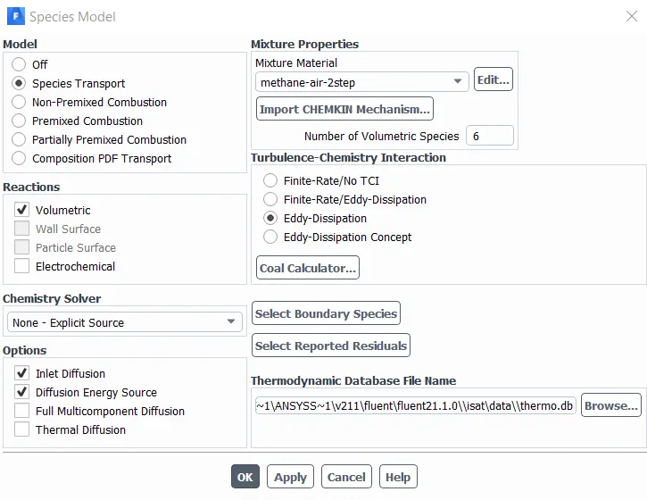
After completing the viscous model selection, the species model can be selected from the model of FLUENT in outline view or can be also select from physics tab > models. As the species model turn on, the energy equation will get turn on automatically. Energy model use to determine the temperature generated during the reaction in species transport equation. In species model, species transport option has to be selected followed by volumetric reaction. The mixture properties should be select one at a time. If user has select any other mixture properties model rather than given one, then that setup need to be reset and again whole process has to be followed accordingly. The mixture model which is used for simulation is ‘methane-air-2step’ in which number of volumetric species are six i.e. CO2, H2O, CH4, N2, O2 and CO. As state earlier this model is governed by effect of turbulence hence Eddy dissipation turbulence-chemistry interaction is selected.
|
Figure 14- Species Model parameter for Simulation |
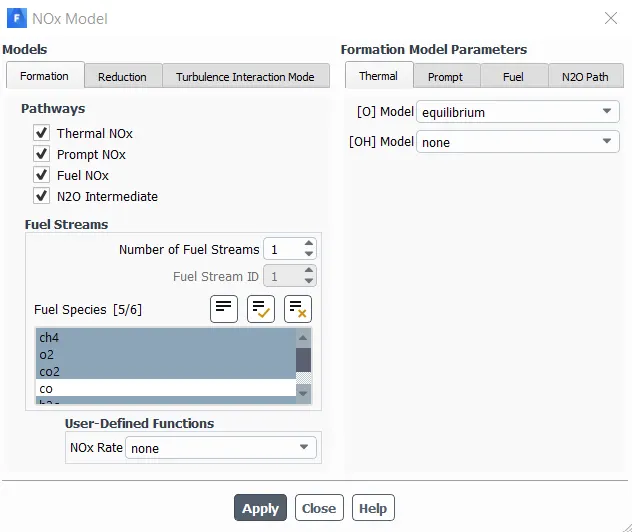
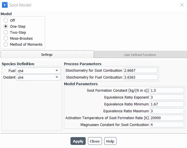
Similar to species model setup, NOx and soot model has to be done accordingly. As discussed earlier the NOx can be produce due to high temperature and rich fuel mixture, hence all the pathways which can track the generation of NOx are activated for the simulation. Similarly, the soot model is also activated in which one-step soot model is used for the tracking of soot generation during the combustion process.
|
Figure 15- NOx Model parameter for Simulation |
|
Figure 16- Soot Model parameter for Simulation |
3.3 Specification of Boundary Condition
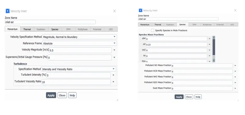
The boundary conditions which are used for this simulation are velocity inlet and pressure outlet with an axis for Axi-symmetric condition. There are two inlets for this simulation. The first velocity inlet is for air which is flowing inside the burner at the speed of 0.5m/sec. The Air is entering at atmospheric pressure inside burner and at 300 kelvin temperature. In species tab of air inlet, it is required to provide information about how much of oxygen is entering in the burner. The 0.23 mass fraction of O2 is coming with air for the reaction purpose. The definition of Air inlet is shown in figure 17.
|
Figure 17- Air-Inlet Boundary Condition specifications |
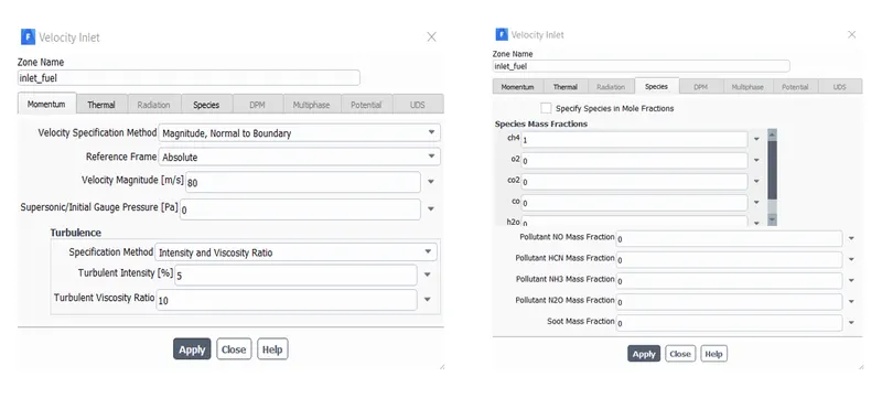
Similarly, for the fuel inlet the momentum boundary conditions are consider are velocity inlet with the value of 80m/sec. The fuel is also entering at atmospheric pressure and 300 kelvin temperature. The most important part of fuel inlet is the specification of species for the simulation. In the species tab of fuel inlet boundary condition the mass fraction of Fuel is defined as 1 of CH4. The information about fuel inlet boundary condition is shown in figure 18.
|
Figure 18- Fuel-Inlet Boundary Condition specifications |
Other than this boundary condition, the pressure outlet boundary condition is kept similar and axis should be put as axis as per the defined by FLUENT automatically.
3.4 Solution Method
Solution method for the simulation is consider as default by FLUENT. Depend upon the version used FLUENT set the solution method as default. As it was found that version from 20 onward the default method of solution method is set as Coupled rather than SIMPLE in previous version. The spatial discretization for all species should be set as second order upwind function. For turbulent Kinetic energy and turbulent dissipation rate same second order upwind function has to be used for better convergence. The convergence factor is also set as default and hybrid initialization method is used to determine the initial value for calculation of whole simulation.
4.0 Simulation Results
4.1 Baseline Mesh Result
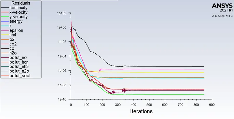
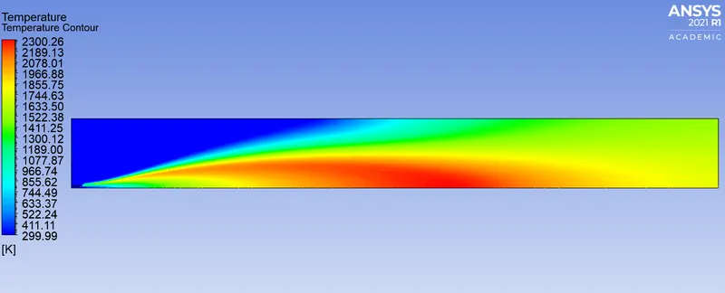
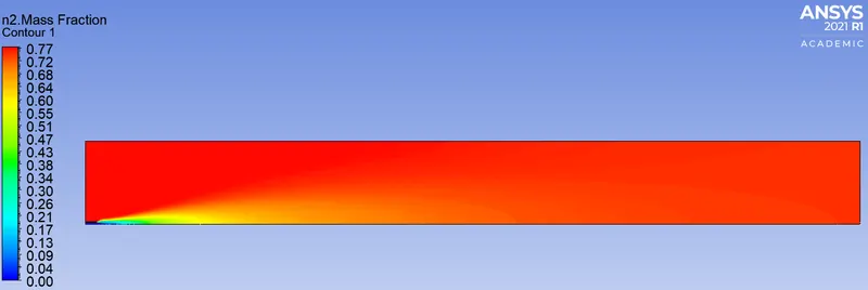
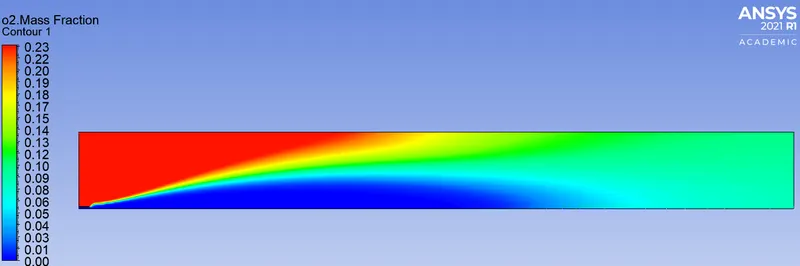
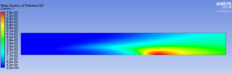
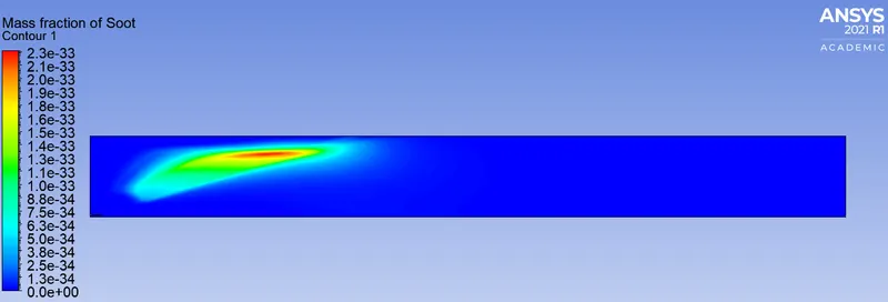
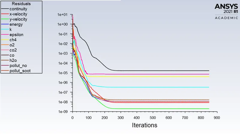
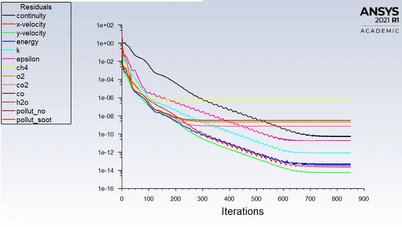
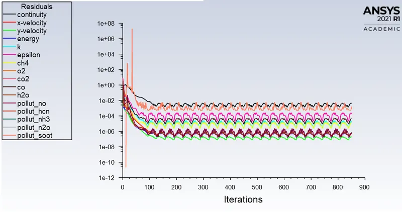
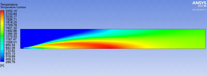
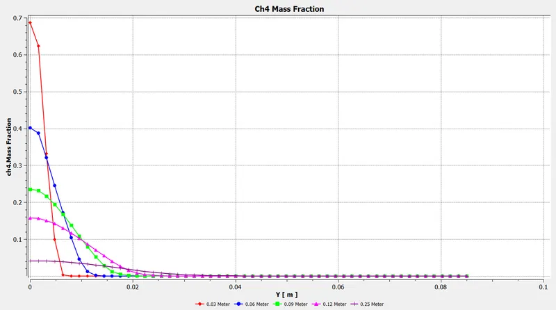
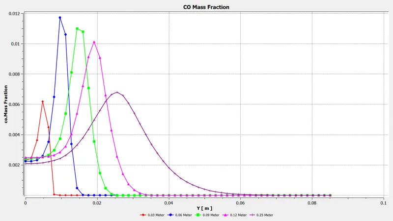
The information which is shared in previous section is applied all the simulation cases except changes in boundary condition of fuel inlet is made for respective further cases. For the baseline mesh setup, the parameters are kept as discussed in boundary condition and simulation is run for the 850 iteration. The data file quantity is setup to read all the results from FLUENT to post-processor. The results of the baseline mesh setup are given below:
1) Residual Plot
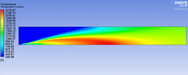
2) Temperature plot
3) Mass fraction of CH4
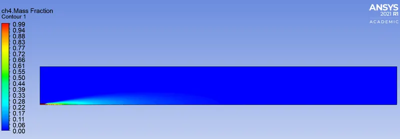
4) Mass Fraction CO
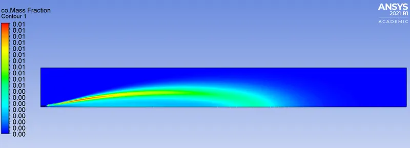
5) Mass Fraction of CO2
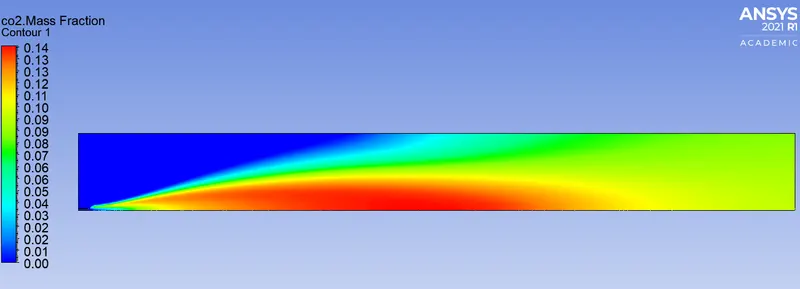
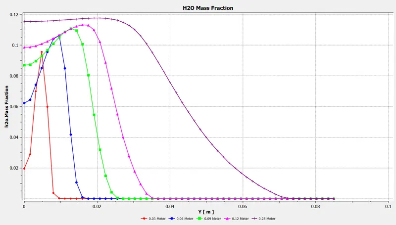
6) Mass Fraction of H2O
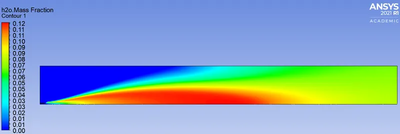
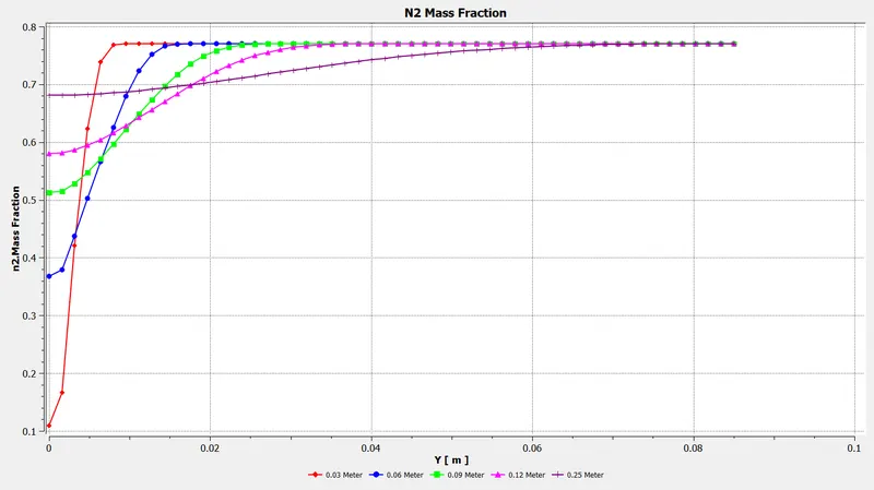
7) Mass Fraction of N2
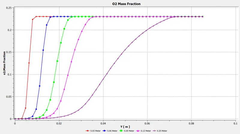
8) Mass Fraction of O2
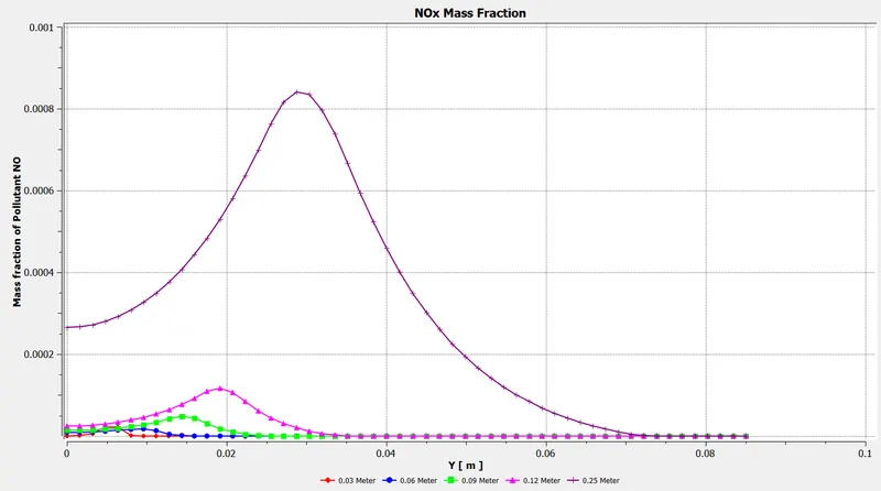
9) Mass fraction of NOx
10) Mass Fraction of Soot
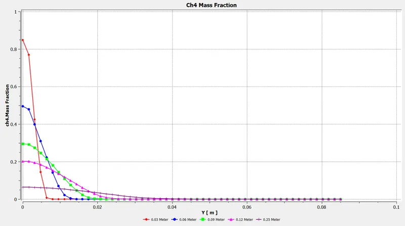
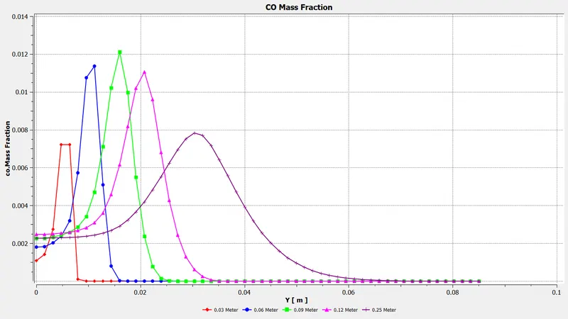
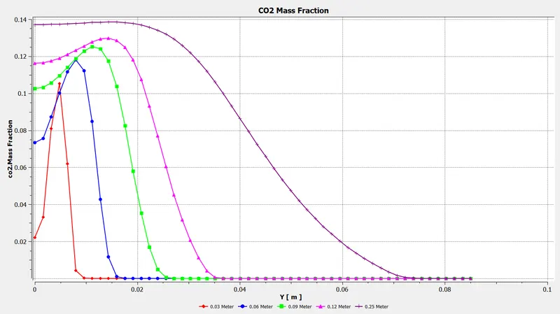
11) Line Plots for graphs
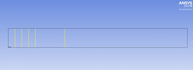
12) Graph of CH4
13) Graph of CO
14) Graph of CO2
15) Graph of H2O
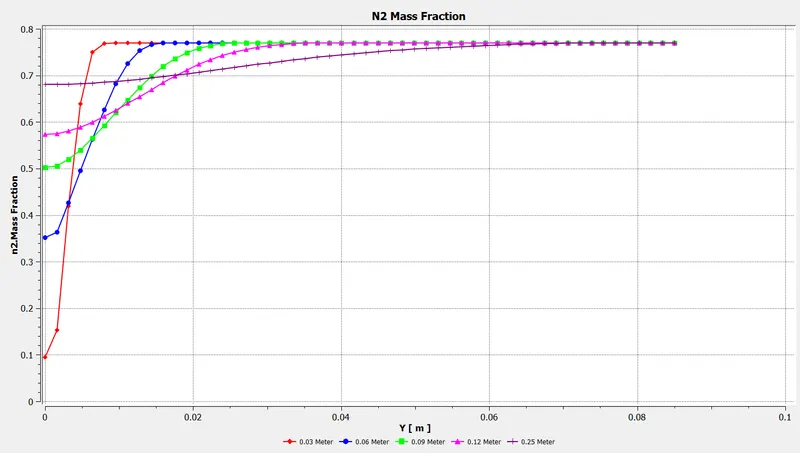
16) Graph of N2
17) Graph of O2
18) Graph of NOx
19) Graph of Soot
4.2 Case 1 - Oxygen 5%
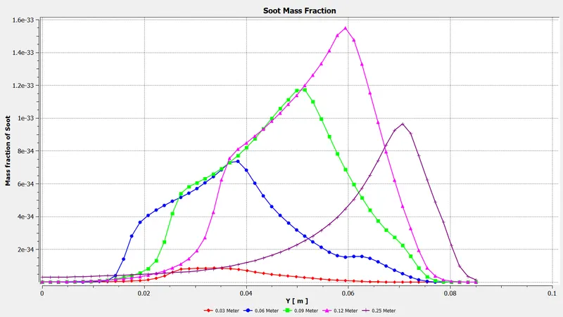
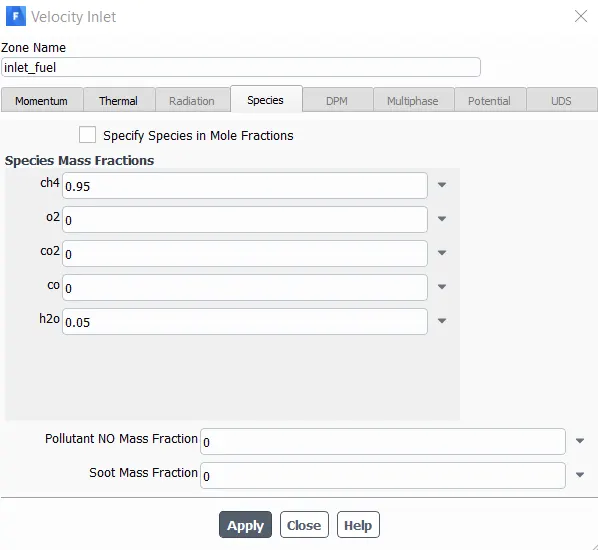
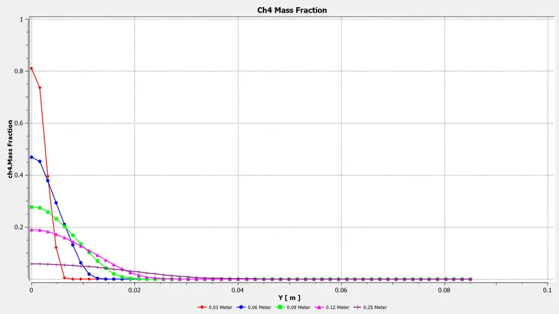
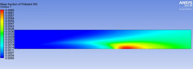
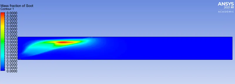
In baseline mesh setup it can be seen that there is proportion of NOx and soot is generated inside the burner. the location of NOx is toward the outlet is more and soot formation is done near the air inlet. To lower the NOx and soot formation in burner the fuel is mixed with Water vapour which entering from same inlet location. For this case only 5% of water is made to mix with fuel and flow at 80m/sec velocity. As the Mass fraction of water is increased in fuel inlet consequently the mass fraction of fuel has to be decrease. The mass fraction of water in this case will be 0.05 whereas mass fraction of fuel will be 0.95.
|
Figure 19- Mass Fraction definition for Case 1 |
1) Residuals
2) Temperature plot
3) Graph of CH4
4) Graph of CO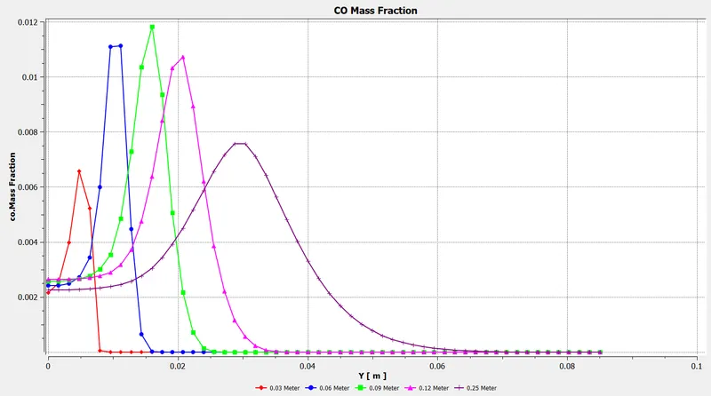
4) Graph of CO2
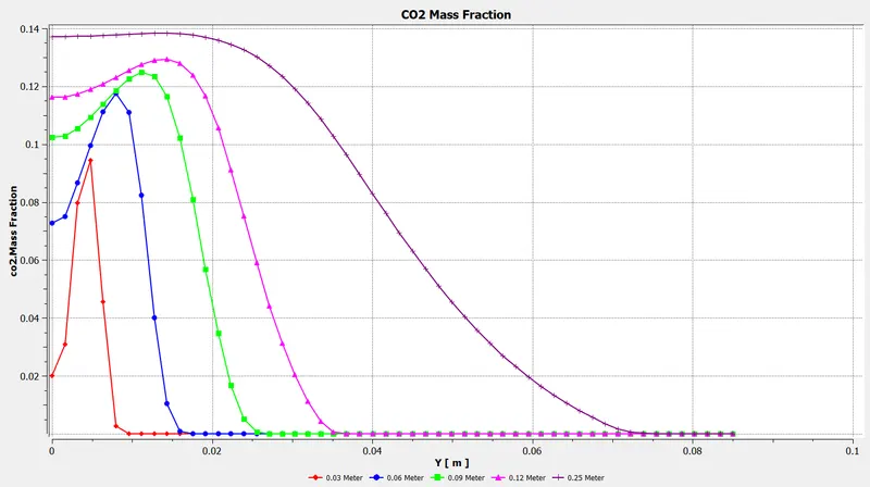
5) Graph of H2O
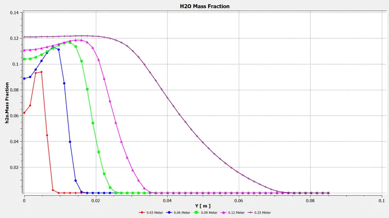
6) Graph of N2
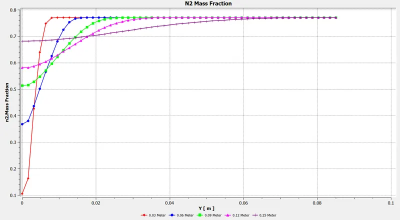
7) Graph of O2
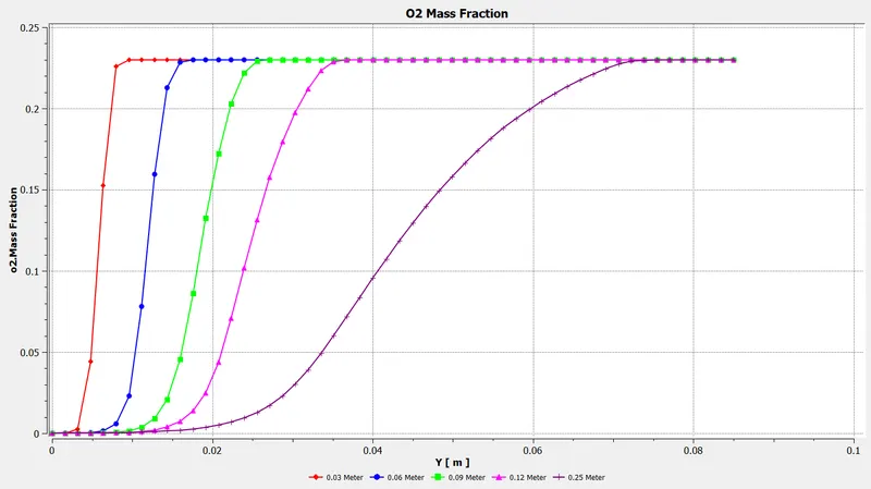
8) Graph of NOx
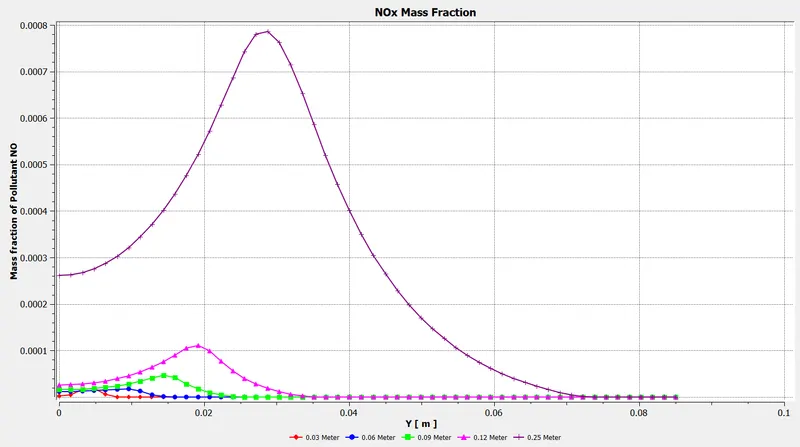
9) Graph of Soot
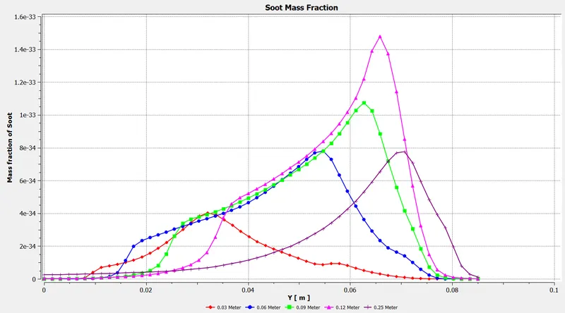
10) Mass Fraction of NOx
11) Mass Fraction of Soot
4.2 Case 2 - Oxygen 10%
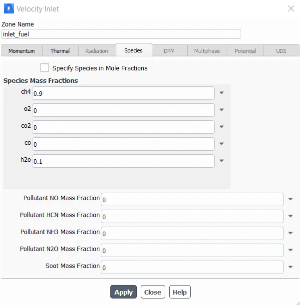
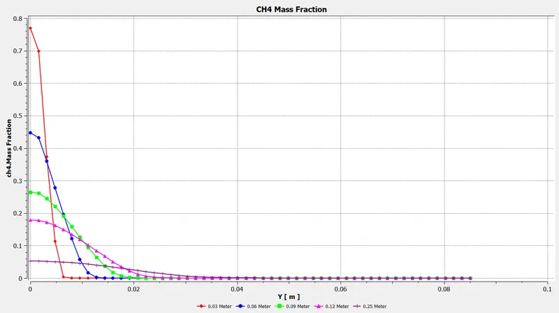
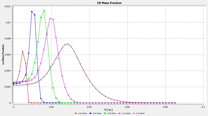
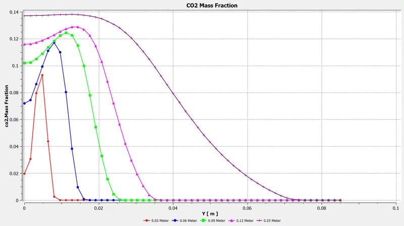
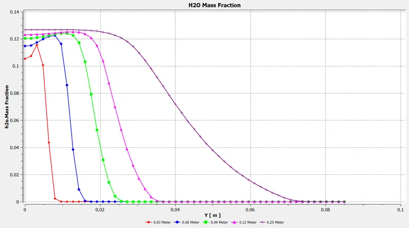
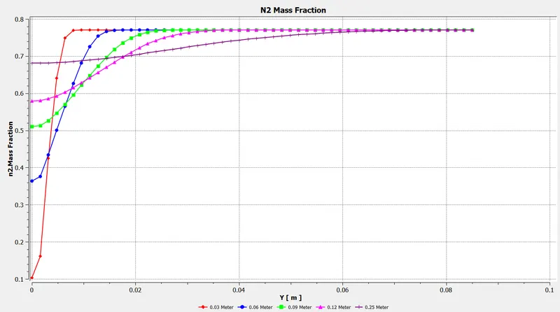
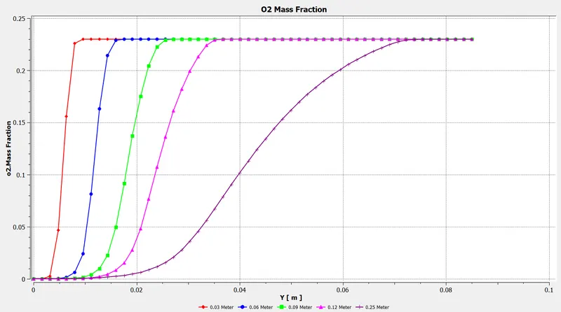
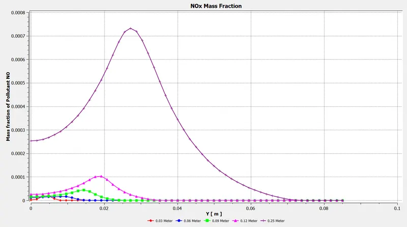
In Case 2 the percentage of oxygen is increased by 5% again. The specification of mass fraction of fuel and water is given figure 20
|
Figure 20- Mass Fraction definition for Case 2 |
1) Residuals
2) Temperature plot
3) Graph of CH4
4) Graph of CO
5) Graph of CO2
6) Graph of H2O
7) Graph of N2
8) Graph of O2
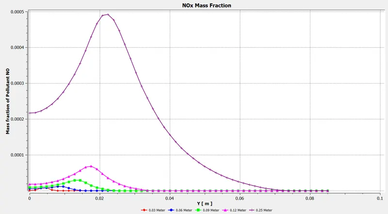
9) Graph of NOx
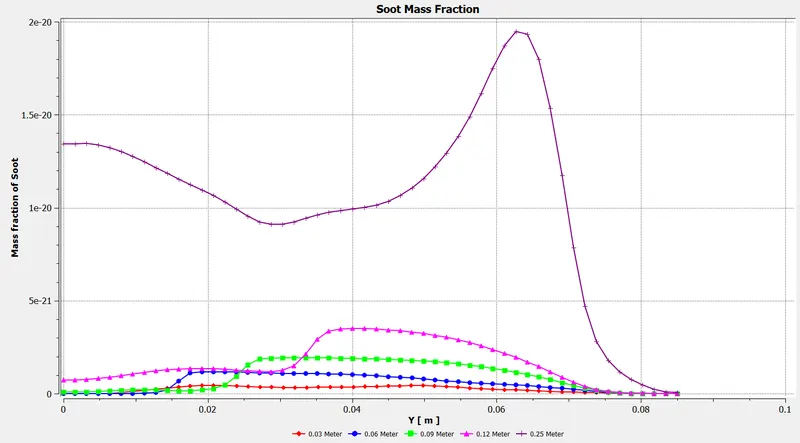
10) Graph of Soot
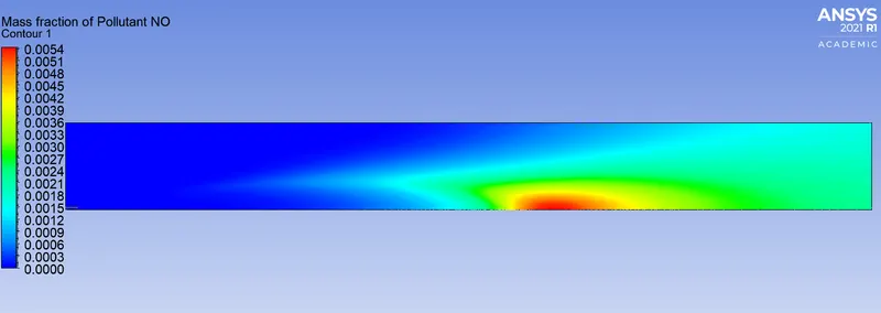
11) Mass Fraction of NOx
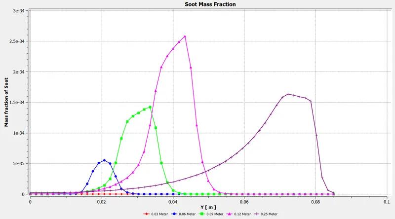
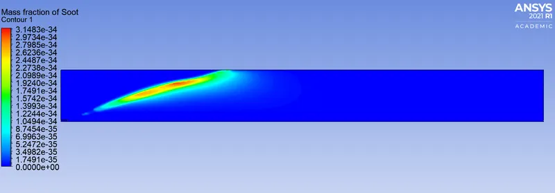
12) Mass Fraction of Soot
4.3 Case 3 - Oxygen 20%
In Case 3 the percentage of oxygen is increased by 10% again. The specification of mass fraction of fuel and water is given figure 21
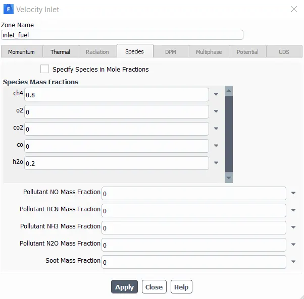
| Figure 21- Mass Fraction definition for Case 3 |
1) Residual
2) Temperature Contour
3) Graph of CH4
4) Graph of CO
5) Graph of CO2
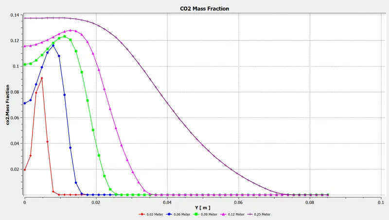
6) Graph of H2O
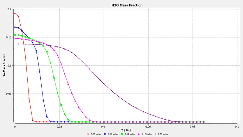
7) Graph of N2
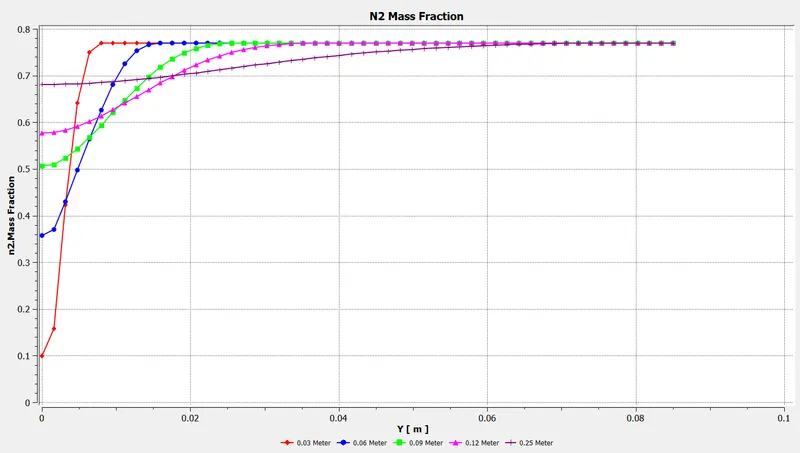
8) Graph of O2
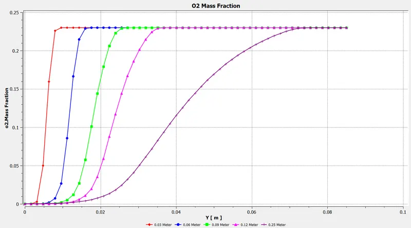
9) Graph of NOx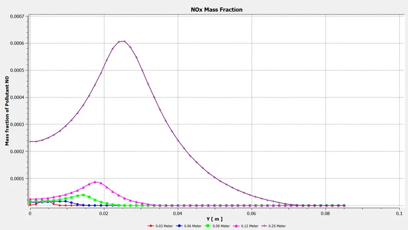
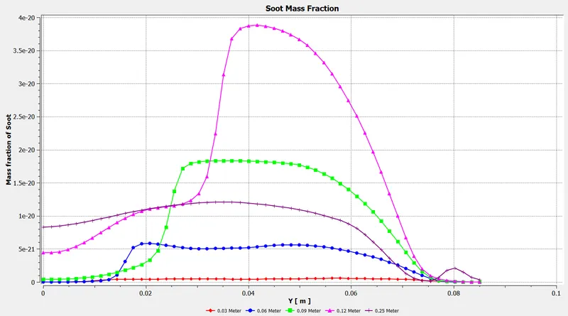
10) Graph of Soot
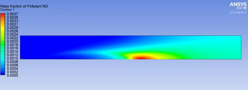
11) Mass Fraction of NOx
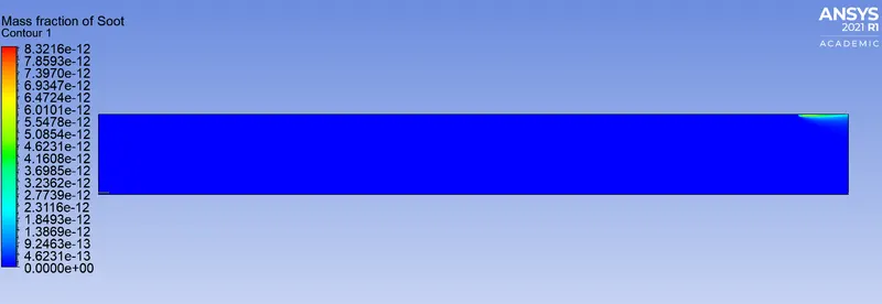
12) Mass Fraction of Soot
4.3 Case 4 - Oxygen 30%
In Case 4 the percentage of oxygen is increased by 10% again. The specification of mass fraction of fuel and water is given figure 22
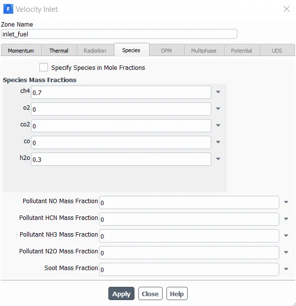
| Figure 22- Mass Fraction definition for Case 4 |
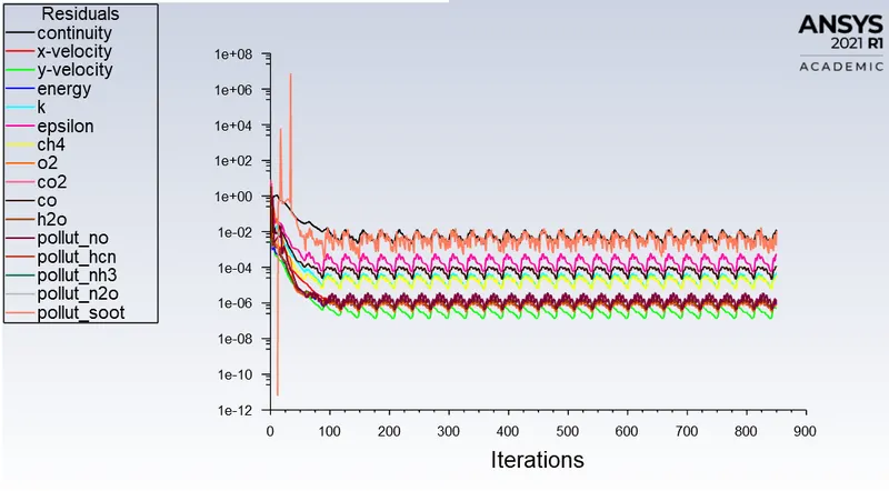
1) Residual
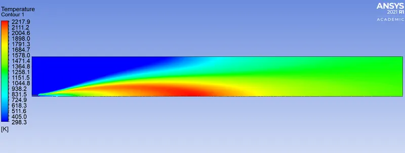
2) Temperature Contour'
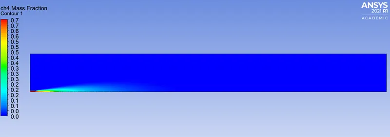
3) Mass Fraction of CH4
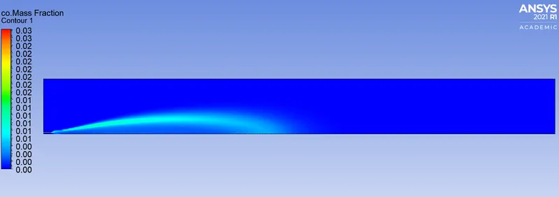
4) Mass Fraction of CO
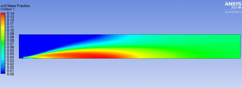
5) Mass Fraction of CO2
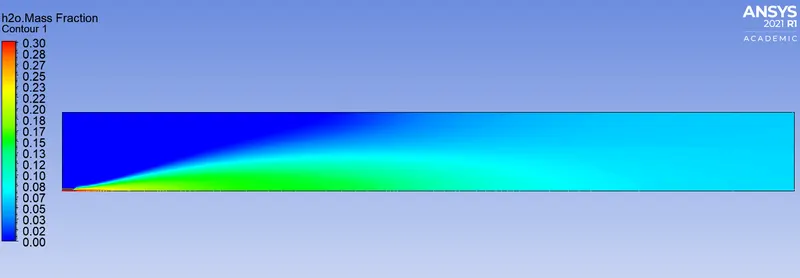
6) Mass Fraction of H2O
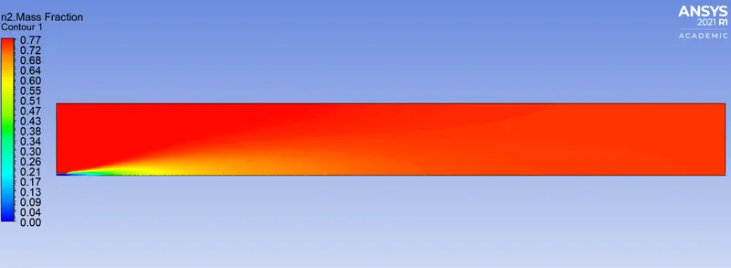
7) Mass Fraction of N2
8) Mass Fraction of O2
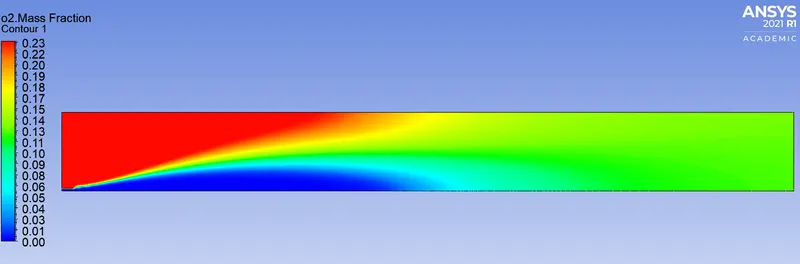
9) Mass Fraction of NOx
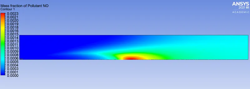
10) Mass Fraction of Soot
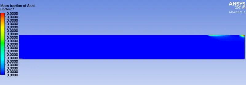
11) Graph of CH4
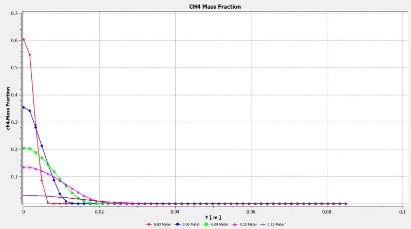
12) Graph of CO
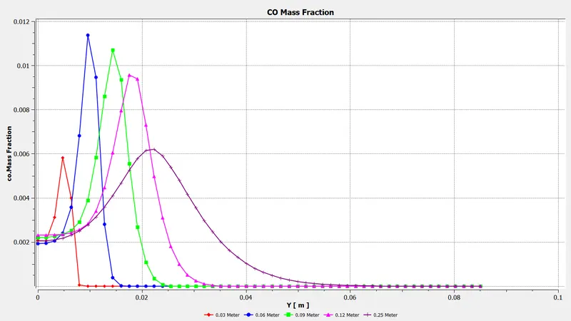
13) Graph of CO2
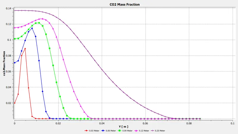
14) Graph of H2O
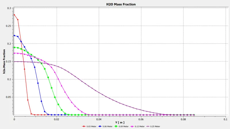
15) Graph of N2
16) Graph of O2
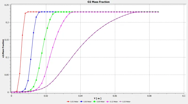
17) Graph of NOx
18) Graph of Soot
5.0 Inference
5.1 Result Table
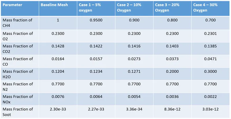
| Table 1 - Result for All the cases of Simulation |
5.2 Conclusion
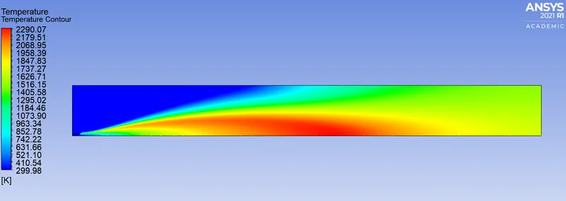
- In baseline mesh setup in which the whole amount of CH4 is present for as the fuel the amount of soot and NOx is greater as compared to other cases. Also the maximum temperature is about 2300 K.
- In next cases where the water is added with fuel in respect of 5% to 30% there is reduction of NOx by certain amount. For case 1 the reduction of NOx is about 15.78%. For case 2 same reduction of NOx is 28.94%. For case 3 the NOx reduction is 52.64% whereas for case 4 the NOx reduction is about 71.05%. Hence adding the water with fuel is considerably decreasing the NOx emissions from the exhaust products.
- Similar to NOx, from the result table it can be seen that the mass fraction of CO2 is also decreasing as water percentage is increasing. The Mass fraction of N2 is almost constant for all the cases which means the flame instability for the burner is almost constant for all the cases of combustion.
- In case of soot formation, it can see that, mass fraction of soot is decreasing for case 1 and 2 but for case 3 and 4 it has increased. After checking the Mass fraction of soot contour for all the cases, it is evident that soot formation from case 1 to 4 is unbalanced but the amount of soot formation is significantly lowered for case 3 and 4. It is seen that from case 3 and 4 contour of mass fraction of soot, the formation of soot is nearer toward the outlet of burner which is common practice of soot to deposited at the outlet.
- From the whole simulation it concluded that providing water with fuel will reduce the harmful exhaust emission such as NOx and Soot.
5.3 References
1) Modelling soot production and thermal radiation for turbulent diffusion flames - ScienceDirect
3) ANSYS FLUENT 12.0 Theory Guide - 13.1.3 Thermal NOx Formation (enea.it)